Overview of statistical learning theory Daniel Hsu Columbia TRIPODS - PowerPoint PPT Presentation
Overview of statistical learning theory Daniel Hsu Columbia TRIPODS Bootcamp 1 Statistical model for machine learning 2 Basic goal of machine learning Goal : Predict outcome y from set of possible outcomes Y , on the basis of observation x
Overview of statistical learning theory Daniel Hsu Columbia TRIPODS Bootcamp 1
Statistical model for machine learning 2
Basic goal of machine learning Goal : Predict outcome y from set of possible outcomes Y , on the basis of observation x from feature space X . ◮ Examples : 1. x = email message, y = spam or ham 2. x = image of handwritten digit, y = digit 3. x = medical test results, y = disease status 3
Basic goal of machine learning Goal : Predict outcome y from set of possible outcomes Y , on the basis of observation x from feature space X . ◮ Examples : 1. x = email message, y = spam or ham 2. x = image of handwritten digit, y = digit 3. x = medical test results, y = disease status Learning algorithm : ◮ Receives training data ( x 1 , y 1 ) , . . . , ( x n , y n ) ∈ X × Y and returns a prediction function ˆ f : X → Y . ◮ On (new) test example ( x, y ) , predict ˆ f ( x ) . 3
Assessing the quality of predictions Loss function : ℓ : Y × Y → R + ◮ Prediction is ˆ y , true outcome is y . ◮ Loss ℓ (ˆ y, y ) measures how bad ˆ y is as a prediction of y . 4
Assessing the quality of predictions Loss function : ℓ : Y × Y → R + ◮ Prediction is ˆ y , true outcome is y . ◮ Loss ℓ (ˆ y, y ) measures how bad ˆ y is as a prediction of y . Examples : 1. Zero-one loss: 0 if ˆ y = y, ℓ (ˆ y, y ) = 1 { ˆ y � = y } = 1 if ˆ y � = y. 2. Squared loss (for Y ⊆ R ): y − y ) 2 . ℓ (ˆ y, y ) = (ˆ 4
Why is this possible? ◮ Only input provided to learning algorithm is training data ( x 1 , y 1 ) , . . . , ( x n , y n ) . ◮ To be useful, training data must be related to test example ( x, y ) . How can we formalize this? 5
Basic statistical model for data IID model of data Regard training data and test example as independent and identically distributed ( X × Y ) -valued random variables: ( X 1 , Y 1 ) , . . . , ( X n , Y n ) , ( X, Y ) ∼ iid P. Can use tools from probability to study behavior of learning algorithms under this model. 6
Risk Loss ℓ ( f ( X ) , Y ) is random, so study average-case performance. Risk of a prediction function f , defined by R ( f ) = E [ ℓ ( f ( X ) , Y )] , where expectation is taken with respect to test example ( X, Y ) . 7
Risk Loss ℓ ( f ( X ) , Y ) is random, so study average-case performance. Risk of a prediction function f , defined by R ( f ) = E [ ℓ ( f ( X ) , Y )] , where expectation is taken with respect to test example ( X, Y ) . Examples : 1. Mean squared error : ℓ = squared loss, R ( f ) = E [( f ( X ) − Y ) 2 ] . 2. Error rate : ℓ = zero-one loss, R ( f ) = P ( f ( X ) � = Y ) . 7
Comparison to classical statistics How (classical) learning theory differs from classical statistics : ◮ Typically, data distribution P is allowed to be arbitrary. ◮ E.g., not from a parametric family { P θ : θ ∈ Θ } . ◮ Focus on prediction rather than general estimation of P . Now : Much overlap between machine learning and statistics. 8
Inductive bias 9
Is predictability enough? Requirements for learning: ◮ Relationship between training data and test example ◮ Formalized by iid model for data. ◮ Relationship between Y and X . ◮ Example: X and Y are non-trivially correlated. Is this enough? 10
No free lunch For any n ≤ |X| 2 and any learning algorithm, there is a distribution, from which the n training data and test example are drawn iid, s.t.: 1. There is a function f ∗ : X → Y with P ( f ∗ ( X ) � = Y ) = 0 . 2. The learning algorithm returns a function ˆ f : X → Y with f ( X ) � = Y ) ≥ 1 P ( ˆ 4 . 11
How to pay for lunch Must make some assumption about learning problem in order for learning algorithm to work well. ◮ Called inductive bias of the learning algorithm. 12
How to pay for lunch Must make some assumption about learning problem in order for learning algorithm to work well. ◮ Called inductive bias of the learning algorithm. Common approach: ◮ Assume there is a good prediction function in a restricted function class F ⊂ Y X . ◮ Goal: find ˆ f : X → Y with small excess risk R ( ˆ f ) − min f ∈F R ( f ) either in expectation or with high probability over random draw of training data. 12
Examples 13
Example #1: Threshold functions X = R , Y = { 0 , 1 } . ◮ Threshold functions F = { f θ : θ ∈ R } where f θ is defined by 0 if x ≤ θ, f θ ( x ) = 1 { x > θ } = 1 if x > θ. 14
Example #1: Threshold functions X = R , Y = { 0 , 1 } . ◮ Threshold functions F = { f θ : θ ∈ R } where f θ is defined by 0 if x ≤ θ, f θ ( x ) = 1 { x > θ } = 1 if x > θ. ◮ Learning algorithm: 1. Sort training examples by x i -value. 2. Consider candidate threshold values that are (i) equal to x i -values, (ii) equal to values midway between consecutive but non-equal x i -values, and (iii) a value smaller than all x i -values. 3. Among candidate thresholds, pick ˆ θ such that f ˆ θ incorrectly classifies the smallest number of examples in training data. 14
Example #2: Linear functions X = R d , Y = R , ℓ = squared loss. ◮ Linear functions F = { f w : w ∈ R d } where f w is defined by f w ( x ) = w T x. 15
Example #2: Linear functions X = R d , Y = R , ℓ = squared loss. ◮ Linear functions F = { f w : w ∈ R d } where f w is defined by f w ( x ) = w T x. ◮ Learning algorithm (“Ordinary Least Squares”): ◮ Return a solution ˆ w to system of linear equations given by n n 1 w = 1 � � T x i x y i x i . i n n i =1 i =1 15
Example #3: Linear classifiers X = R d , Y = {− 1 , +1 } . ◮ Linear classifiers F = { f w : w ∈ R d } where f w is defined by − 1 if w T x ≤ 0 , f w ( x ) = sign( w T x ) = +1 if w T x > 0 . 16
Example #3: Linear classifiers X = R d , Y = {− 1 , +1 } . ◮ Linear classifiers F = { f w : w ∈ R d } where f w is defined by − 1 if w T x ≤ 0 , f w ( x ) = sign( w T x ) = +1 if w T x > 0 . ◮ Learning algorithm (“Support Vector Machine”): ◮ Return solution ˆ w to following optimization problem: n 2 + 1 λ � 2 � w � 2 min [1 − y i w T x i ] + . n w ∈ R d i =1 16
Over-fitting and generalization 17
Over-fitting Over-fitting : Phenomenon where learning algorithm returns ˆ f that “fits” training data well, but does not give accurate predictions on test examples. 18
Over-fitting Over-fitting : Phenomenon where learning algorithm returns ˆ f that “fits” training data well, but does not give accurate predictions on test examples. ◮ Empirical risk of f (on training data ( X 1 , Y 1 ) , . . . , ( X n , Y n ) ): n R n ( f ) = 1 � ℓ ( f ( X i ) , Y i ) . n i =1 ◮ Over-fitting : R n ( ˆ f ) small, but R ( ˆ f ) large. 18
Generalization How to avoid over-fitting “Theorem”: R ( ˆ f ) − R n ( ˆ f ) is likely to be small, if learning algorithm chooses ˆ f from F that is “not too rich” relative to n . ◮ ⇒ Observed performance on training data (i.e., empirical risk) generalizes to expected performance on test example (i.e., risk). ◮ Justifies learning algorithms based on minimizing empirical risk. 19
Other issues 20
Risk decomposition R ( ˆ f ) = g : X→Y R ( g ) inf (inherent unpredictability) + inf f ∈F R ( f ) − g : X→Y R ( g ) inf (approximation gap) + inf f ∈F R n ( f ) − inf f ∈F R ( f ) (estimation gap) + R n ( ˆ f ) − inf f ∈F R n ( f ) (optimization gap) + R ( ˆ f ) − R n ( ˆ f ) . (more estimation gap) 21
Risk decomposition R ( ˆ f ) = g : X→Y R ( g ) inf (inherent unpredictability) + inf f ∈F R ( f ) − g : X→Y R ( g ) inf (approximation gap) + inf f ∈F R n ( f ) − inf f ∈F R ( f ) (estimation gap) + R n ( ˆ f ) − inf f ∈F R n ( f ) (optimization gap) + R ( ˆ f ) − R n ( ˆ f ) . (more estimation gap) ◮ Approximation : ◮ Which function classes F are “rich enough” for a broad class of learning problems? ◮ E.g., neural networks, Reproducing Kernel Hilbert Spaces. ◮ Optimization : ◮ Often finding minimizer of R n is computationally hard. ◮ What can we do instead? 21
Alternative model: online learning Alternative to iid model for data : ◮ Examples arrive in a stream, one at at time. ◮ At time t : ◮ Nature reveals x t . ◮ Learner makes prediction ˆ y t . ◮ Nature reveals y t . ◮ Learner incurs loss ℓ (ˆ y t , y t ) . 22
Alternative model: online learning Alternative to iid model for data : ◮ Examples arrive in a stream, one at at time. ◮ At time t : ◮ Nature reveals x t . ◮ Learner makes prediction ˆ y t . ◮ Nature reveals y t . ◮ Learner incurs loss ℓ (ˆ y t , y t ) . Relationship between past and future : ◮ No statistical assumption on data. ◮ Just assume there exists f ∗ ∈ F with small (empirical) risk n 1 ℓ ( f ∗ ( x t ) , y t ) . � n t =1 22
Recommend
More recommend
Explore More Topics
Stay informed with curated content and fresh updates.
