Statistical and Computational Statistical and Computational - PowerPoint PPT Presentation

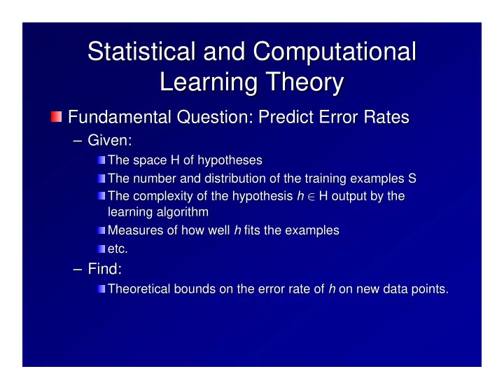
Statistical and Computational Statistical and Computational Learning Theory Learning Theory Fundamental Question: Predict Error Rates Fundamental Question: Predict Error Rates – Given: Given: – The space H of hypotheses The space H of hypotheses The number and distribution of the training examples S The number and distribution of the training examples S h ∈ ∈ H output by the The complexity of the hypothesis h H output by the The complexity of the hypothesis learning algorithm learning algorithm Measures of how well h h fits the examples fits the examples Measures of how well etc. etc. – Find: Find: – Theoretical bounds on the error rate of h h on new data points. on new data points. Theoretical bounds on the error rate of

General Assumptions General Assumptions (Noise- -Free Case) Free Case) (Noise Assumption: Examples are generated according to a Assumption: Examples are generated according to a probability distribution D( x ) and labeled according to an probability distribution D( x ) and labeled according to an unknown function f: y y = f( = f( x ) unknown function f: x ) Learning Algorithm: The learning algorithm is given a Learning Algorithm: The learning algorithm is given a set of m m examples, and it outputs an hypothesis examples, and it outputs an hypothesis h h ∈ ∈ H H set of that is consistent consistent with those examples (i.e., correctly with those examples (i.e., correctly that is classifies all of them). classifies all of them). ε on new examples should have a low error rate ε Goal: h h should have a low error rate on new examples Goal: drawn from the same distribution same distribution D. D. drawn from the h f error ( h, f ) = P D [ f ( x ) 6 = h ( x )]

Probably- -Approximately Correct Approximately Correct Probably Learning Learning δ We allow our algorithms to fail with probability δ We allow our algorithms to fail with probability Imagine drawing a sample of m m examples, running the examples, running the Imagine drawing a sample of learning algorithm, and obtaining h h . Sometimes, the . Sometimes, the learning algorithm, and obtaining sample will be unrepresentative, so we only want to sample will be unrepresentative, so we only want to – δ δ of the time, the hypothesis will have error insist that 1 – of the time, the hypothesis will have error insist that 1 ε . For example, we might want to obtain a less than ε . For example, we might want to obtain a less than 99% accurate hypothesis 90% of the time. 99% accurate hypothesis 90% of the time. Let P m m (S) be the probability of drawing data set S of m m Let P D (S) be the probability of drawing data set S of D examples according to D. examples according to D. P m D [ error ( f, h ) > ² ] < δ

Case 1: Finite Hypothesis Space Case 1: Finite Hypothesis Space Assume H is finite is finite Assume H ε . What is ) > ε ∈ H such that Consider h h 1 1 ∈ H such that error error ( ( h h , , f f ) > . What is Consider the probability that it will correctly classify m m the probability that it will correctly classify training examples? training examples? If we draw one one training example, ( training example, ( x , y y 1 ), what is If we draw 1 , 1 ), what is x 1 the probability that h h 1 classifies it correctly? the probability that 1 classifies it correctly? – ε ε ) P[h 1 ( x ) = y y 1 ] = (1 – ) P[h 1 ( 1 ) = 1 ] = (1 x 1 What is the probability that h h will be right will be right m m What is the probability that times? times? - ε ε ) m m P m [h 1 ( x ) = y y 1 ] = (1 - ) m P D [h 1 ( 1 ) = 1 ] = (1 x 1 D

Finite Hypothesis Spaces (2) Finite Hypothesis Spaces (2) Now consider a second hypothesis h h 2 that is Now consider a second hypothesis 2 that is ε - also ε -bad. What is the probability that bad. What is the probability that either either h h 1 also 1 or h h 2 will survive the m m training examples? training examples? or 2 will survive the m m P m [ h h 1 1 ∨ ∨ h h 2 survives] = P m [ h h 1 survives] + P D [ 2 survives] = P D [ 1 survives] + D D m P m [ h h 2 survives] – – P D [ 2 survives] D m ∧ h P m [h 1 1 ∧ h 2 survives] P D [h 2 survives] D · P P m m survives] + P m m · [ h h 1 [ h h 2 survives] D [ 1 survives] + P D [ 2 survives] D D – ε ε ) · 2(1 ) m m · 2(1 – k ε ε - So if there are k -bad hypotheses, the bad hypotheses, the So if there are · probability that any one any one of them will survive is of them will survive is · probability that – ε ε ) m k (1 – ) m k (1 – ε ε ) · |H|(1 m Since k k < |H|, this is < |H|, this is · |H|(1 – ) m Since

Finite Hypothesis Spaces (3) Finite Hypothesis Spaces (3) · ε ε · – ε ε ) ε – ε · 1, (1 · e e – Fact: When 0 · 1, (1 – ) · Fact: When 0 therefore therefore m · – ε ε ) ε m – ε · |H| m |H|(1 – ) m |H| e e – |H|(1

Blumer Bound Blumer Bound (Blumer, Ehrenfeucht, Haussler, Warmuth) (Blumer, Ehrenfeucht, Haussler, Warmuth) Lemma. For a finite hypothesis space H, given Lemma. For a finite hypothesis space H, given a set of m m training examples drawn training examples drawn a set of independently according to D, the probability independently according to D, the probability h ∈ ∈ H with true that there exists an hypothesis h H with true that there exists an hypothesis ε consistent with the training error greater than ε consistent with the training error greater than ε m – ε m . e – examples is less than |H| e . examples is less than |H| We want to ensure that this probability is less We want to ensure that this probability is less δ . than δ . than m · · δ δ ε m – ε |H| e e – |H| This will be true when This will be true when µ ¶ m ≥ 1 ln | H | + ln 1 . ² δ

Finite Hypothesis Space Bound Finite Hypothesis Space Bound h ∈ ∈ H is consistent with all Corollary: If h H is consistent with all m m Corollary: If examples drawn according to D, then the examples drawn according to D, then the ε on new data points can be error rate ε on new data points can be error rate estimated as estimated as µ ¶ ² = 1 ln | H | + ln 1 . m δ

Examples Examples Boolean conjunctions over n n features. features. Boolean conjunctions over |H| = 3 n n , since each feature can appear as ¬ x , since each feature can appear as x x j , ¬ x j , or be |H| = 3 j , j , or be missing. missing. µ ¶ ² = 1 n ln3 + ln 1 m δ k- -DNF formulas: DNF formulas: k ∧ x ∨ ( ∧ ¬ ¬ x ∨ ( ∧ x ( x x 1 1 ∧ x 3 ) ∨ ( x x 2 2 ∧ x 4 ) ∨ ( x x 1 1 ∧ x 4 ) ( 3 ) 4 ) 4 ) k disjunctions, so There are at most (2n) k disjunctions, so There are at most (2n) k (2n)k · 2 2 (2n) |H| · |H| for fixed fixed k k , this gives , this gives for k log 2 |H| = (2n) k log 2 |H| = (2n) which is polynomial in n n : : which is polynomial in µ ¶ ² = 1 n k + ln 1 mO δ

Finite Hypothesis Space: Finite Hypothesis Space: Inconsistent Hypotheses Inconsistent Hypotheses Suppose that h h does not perfectly fit the does not perfectly fit the Suppose that data, but rather that it has an error rate of data, but rather that it has an error rate of ε T ε . Then the following holds: T . Then the following holds: v u t ln | H | + ln 1 u δ ² < = ² T + 2 m This makes it clear that the error rate on This makes it clear that the error rate on the test data is usually going to be larger the test data is usually going to be larger ε T than the error rate ε on the training data. than the error rate T on the training data.

Case 2: Infinite Hypothesis Spaces Case 2: Infinite Hypothesis Spaces and the VC Dimension and the VC Dimension Most of our classifiers (LTUs, neural networks, SVMs) Most of our classifiers (LTUs, neural networks, SVMs) have continuous parameters and therefore, have infinite have continuous parameters and therefore, have infinite hypothesis spaces hypothesis spaces Despite their infinite size, they have limited expressive Despite their infinite size, they have limited expressive power, so we should be able to prove something power, so we should be able to prove something Definition: Consider a set of m m examples S = {( examples S = {( x ,y 1 ) , , … …, , Definition: Consider a set of 1 ,y 1 ) x 1 ( x ,y m )} . . An hypothesis space H can An hypothesis space H can trivially fit trivially fit S, if for S, if for ( m ,y m )} x m every possible way of labeling the examples in S, there every possible way of labeling the examples in S, there h ∈ ∈ H that gives this labeling. (H is said to exists an h H that gives this labeling. (H is said to exists an “shatter shatter” ” S) S) “ Definition: The Vapnik Vapnik- -Chervonenkis Chervonenkis dimension (VC dimension (VC- - Definition: The dimension) of an hypothesis space H is the size of the dimension) of an hypothesis space H is the size of the largest set S of examples that can be trivially fit by H. largest set S of examples that can be trivially fit by H. · log For finite H, VC(H) · log 2 |H| For finite H, VC(H) 2 |H|