Overview Decision Theory Classification and Bayes decision rule - PowerPoint PPT Presentation
Overview Decision Theory Classification and Bayes decision rule Sampling vs diagnostic paradigm Chris Williams Classification with Gaussians Loss, Utility and Risk School of Informatics, University of Edinburgh Reject option October 2010
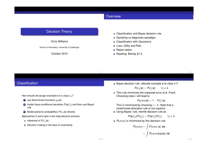
Overview Decision Theory Classification and Bayes decision rule Sampling vs diagnostic paradigm Chris Williams Classification with Gaussians Loss, Utility and Risk School of Informatics, University of Edinburgh Reject option October 2010 Reading: Bishop §1.5 1 / 15 2 / 15 Classification Bayes decision rule: allocate example x to class k if P ( C k | x ) > P ( C j | x ) ∀ j � = k This rule minimizes the expected error at x . Proof: How should we assign example x to a class C k ? Choosing class i will lead to use discriminant functions y k ( x ) 1 P ( error | x ) = 1 − P ( C i | x ) model class-conditional densities P ( x |C k ) and then use Bayes’ 2 This is minimized by choosing i = k . Note that a rule randomized allocation rule is not superior. Using Bayes’ rule, rewrite decision rule as Model posterior probabilities P ( C k | x ) directly 3 Approaches 2 and 3 give a two-step decision process P ( x |C k ) P ( C k ) > P ( x |C j ) P ( C j ) ∀ j � = k Inference of P ( C k | x ) P ( error ) is minimized by this decision rule � Decision making in the face of uncertainty P ( error ) = P ( error , x ) d x � = P ( error | x ) p ( x ) d x 3 / 15 4 / 15
Model P ( C k | x ) or P ( x |C k ) ? Diagnostic paradigm (discriminative): Model P ( C k | x ) Errors in classification arise from directly Sampling paradigm (generative): Model P ( x |C k ) and P ( C k ) Errors due to class overlap 1 Pros/cons of diagnostic paradigm: these are unavoidable Modelling P ( C k | x ) can be simpler than modelling Errors resulting from an incorrect decision rule 2 class-conditional densities. use the correct rule! Less sensitive to modelling assumptions as what we need, Errors resulting from an inaccurate model of the posterior 3 P ( C k | x ) is modelled directly probabilities Marginal density p ( x ) is needed to handle outliers and accurate modelling is a challenging problem missing values Use of unclassified observations difficult in diagnostic paradigm Dealing with missing inputs is difficult 5 / 15 6 / 15 Classification with Gaussians class−conditional density 1.4 1.2 Check if 1 P ( C 1 | x ) P ( C 2 | x ) = p ( x |C 1 ) P ( C 1 ) 0.8 p ( x |C 2 ) P ( C 2 ) ≷ 1 0.6 0.4 or if 0.2 ∆( x ) = log p ( x |C 1 ) P ( C 1 ) 0 p ( x |C 2 ) P ( C 2 ) ≷ 0 0 0.5 1 1.5 2 2.5 3 3.5 4 x posterior probability 1 For Gaussian class-conditional densities and Σ 1 = Σ 2 we obtain 0.8 0.6 ( µ 1 − µ 2 ) T Σ − 1 x + 1 1 Σ − 1 µ 1 ) + ln P ( C 1 ) 2 ( µ T 2 Σ − 1 µ 2 − µ T P ( C 2 ) ≷ 0 0.4 0.2 This is a linear classifier 0 0 0.5 1 1.5 2 2.5 3 3.5 4 x For Σ 1 � = Σ 2 , boundaries are hyperquadrics 7 / 15 8 / 15
Example loss function Loss and Risk Patients are classified to classes C 1 = healthy, C 2 = tumour. Actions are a 1 = discharge the patient, a 2 = operate Actions a 1 , . . . , a A might be taken. Given x , which one should be taken? Assume L 11 = L 22 = 0, L 12 = 1 and L 21 = 10, i.e. it is 10 times worse to discharge the patient when they have a tumour than to L ji is the loss incurred if action a i is taken when the state of operate when they do not nature is C j The expected loss (or risk) of taking action a i given x is R ( a 1 | x ) = L 11 P ( C 1 | x ) + L 21 P ( C 2 | x ) = L 21 P ( C 2 | x ) R ( a 2 | x ) = L 12 P ( C 1 | x ) + L 22 P ( C 2 | x ) = L 12 P ( C 1 | x ) � R ( a i | x ) = L ji P ( C j | x ) j Choose action a 1 when R ( a 1 | x ) < R ( a 2 | x ) , i.e. when Choose action k if L 21 P ( C 2 | x ) < L 12 P ( C 1 | x ) � � L jk P ( C j | x ) < L ji P ( C j | x ) ∀ i � = k or P ( C 2 | x ) > L 21 P ( C 1 | x ) j j = 10 L 12 Let a ( x ) = argmin i R ( a i | x ) If L 21 = L 12 = 1 then threshold is 1; in our case we require Overall risk R stronger evidence in favour of C 1 = healthy in order to discharge � R = R ( a ( x ) | x ) p ( x ) d x the patient 9 / 15 10 / 15 Loss−adjusted Decision Boundary Adjusted Normal In credit risk assignment, losses are monetary Note that rescaling loss matrix does not change the decision Minimum classification error is obtained by L ji = 1 − δ ji 11 / 15 12 / 15
Utility and Loss Reject option Basically same thing with opposite sign. Maximize P ( error | x ) = 1 − max P ( C j | x ) j expected utility, minimize expected loss. See Russell and Norvig ch 16 for a discussion of If we can reject some examples, reject those that are most fundamentals of utility theory, and utility of money [not confusable, i.e. where P ( error | x ) is highest examinable] Choose a threshold θ and reject if Russell and Norvig ch 17 discuss sequential decision problems. Involves utilities, uncertainty and sensing; max P ( C j | x ) < θ generalizes problems of planning and search. See RL j course. Gives rise to error-reject curves as θ is varied from 0 to 1 13 / 15 14 / 15 Error-reject curve 100 30 90 25 80 70 20 % Rejected % Incorrect 60 50 15 40 10 30 20 5 10 0 0 0.4 0.6 0.8 1 0 20 40 60 80 100 θ % Rejected 15 / 15
Recommend
More recommend
Explore More Topics
Stay informed with curated content and fresh updates.
