Bayesian Decision Theory with applications to Experimental Design - PowerPoint PPT Presentation

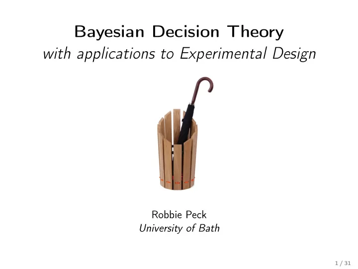
Bayesian Decision Theory with applications to Experimental Design Robbie Peck University of Bath 1 / 31

Overview Bayesian Decision Theory through example Motivating Example Ingredients Special cases Gain functions Bayes Decision Rule Dynamic Programming: Sequential Decision Theory Application to Experimental Design Setting the picture of a Phase II/III program Decision 2 Decision 1 2 / 31

The Umbrella Conundrum ◮ You can take the umbrella, or not take it. ◮ It may or may not rain during the day. ◮ Do not take the umbrella, and it rains → you get wet. ◮ Take the umbrella, and it does not rain → you have to carry it around all day. ◮ You may look at the sky, or see the weather forecast, which may help inform your decision. 3 / 31

Ingredients State of Nature θ ∈ Θ , with associated prior π θ ( · ) Data x ∈ X , with likelihood π x ( · ; θ ) The state of nature is unknown, and the observed data may depend upon the state of nature. Action α ∈ A Decision Rule d : X → A The decision rule stipulates which action to take given observed data. 4 / 31

Ingredients In the umbrella example, State of Nature: Θ := { rain occurs, rain does not occur } Data X := { no clouds, few clouds, many clouds } , or [ 0 , 1 ] Action A := { take umbrella, do not take umbrella } Decision Rule d : X → A d ( x ) = take umbrella ∀ x d ( x ) = do not take umbrella ∀ x � take umbrella if x ∈ { few clouds , many clouds } d ( x ) = do not take umbrella if x = no clouds 5 / 31

No data, Equally weighted losses case... Suppose we have no data X . Further, suppose there is a bijection γ : A → Θ between actions and states of nature, with incorrect actions weighted equally. i.e. α = take umbrella ⇒ γ ( α ) = rain . 6 / 31

No data, Equally weighted losses case... Suppose we have no data X . Further, suppose there is a bijection γ : A → Θ between actions and states of nature, with incorrect actions weighted equally. i.e. α = take umbrella ⇒ γ ( α ) = rain . Optimal Decision rule d : Take action α ⇔ α maximises π θ ( γ ( α )) i.e. Assuming the prior gives a weighting of π θ ( rain ) < 0 . 5 , we never take the umbrella! 7 / 31

... suppose we have data The posterior probability may govern our decision: π ( θ | x ) = π x ( x | θ ) π θ ( θ ) π ( x ) π x ( x | θ ) π θ ( θ ) = � Θ π x ( x | θ ) π θ ( θ ) d θ 8 / 31

... suppose we have data The posterior probability may govern our decision: π ( θ | x ) = π x ( x | θ ) π θ ( θ ) π ( x ) π x ( x | θ ) π θ ( θ ) = � Θ π x ( x | θ ) π θ ( θ ) d θ By minimising the average probability of error � ∞ P ( error ) = P ( error | x ) π ( x ) dx , (1) −∞ one obtains d ( x ) = argmax π ( γ ( α ) | x ) . α ∈A Likelihoods uniform ⇒ decision relies only on priors . Uniform prior ⇒ decision relies only on likelihood . (Bayes decision rule in the case of equal losses) 9 / 31

The need for gain functions ... but not taking an umbrella when it rains is worse than taking an umbrella when it does not rain! We introduce gain functions to complete our theory. 10 / 31

Gain functions The gain function describes the gain of each action. G ( α ; θ ) : A × Θ → R , is the gain incurred by taking action α when the state of nature is θ . In the case of equal costs , G ( α i , θ j ) = δ i , j for suitably ordered α and θ . The expected gain G : A → R , given observed data x is defined as � G ( α | x ) = G ( α | θ ) π ( θ | x ) d θ (2) Θ 11 / 31

Bayes Decision Rule Defining the overall gain of a decision rule as � G ( d ( x ) | x ) π ( x ) dx , (3) X choosing decision rule d such that the overall gain is maximised gives us Bayes Decision Rule : d ( x ) = argmax G ( α | x ) α ∈A (4) � = argmax G ( α | θ ) π ( θ | x ) d θ α ∈A Θ 12 / 31

Back to the umbrella problem ◮ Prior on the state of nature � 0 . 25 if θ = { rain occurs } π θ ( θ ) = 0 . 75 if θ = { no rain occurs} ◮ Gain function G ( · , · ) takes the following form: Action α take umbrella do not take umbrella it rains -0.1 -1 θ no rain -0.1 0 13 / 31

Back to the umbrella problem ◮ We observe some data x ∈ X relating to the prevalence of clouds in the sky on the continuous scale of 0 to 1. ◮ Likelihood of cloud prevalence x ∈ X = [ 0 , 1 ] given θ is: 14 / 31

Bayes decision rule in this case is � d ( x ) = argmax G ( α | θ ) π ( θ | x ) (5) α ∈A θ ∈{ rain, no rain } � �� � ( ∗ ) 15 / 31

Bayes decision rule in this case is � d ( x ) = argmax G ( α | θ ) π ( θ | x ) (5) α ∈A θ ∈{ rain, no rain } � �� � ( ∗ ) Plotting ( ∗ ) for each α ∈ A , 16 / 31

Bayes decision rule in this case is � d ( x ) = argmax G ( α | θ ) π ( θ | x ) (5) α ∈A θ ∈{ rain, no rain } � �� � ( ∗ ) Plotting ( ∗ ) for each α ∈ A , Thus Bayes decision rule is � take umbrella if x ≥ 0 . 4 d ( x ) = if x < 0 . 4 . do not take umbrella 17 / 31

The sequential decision problem When making decisions sequentially, decisions you make at each stage ◮ determine interim loss or gain, and ◮ affect the ability to make decisions at further stages. 18 / 31

The sequential decision problem Dynamic programming (or backward induction) approach: Find the optimal decision rule at the last stage , then work backwards stage by stage, keeping track of the optimal decision rule and the expected payoff when this rule is applied in each stage. 19 / 31

Setting the picture of a Phase II/III program Often we have several treatments that show promise. Require a program that: ◮ Selects the most promising treatment (Phase II). ◮ Build up evidence of the efficacy of the treatment (Phase III). Optimising the overall program is a complicated problem. i.e. the best way to design Phase II depends on how one uses the results of Phase II in designing Phase III. 20 / 31

Phase III design, given Phase II data. Phase II design. 21 / 31

Phase III design, given Phase II data. Phase II design. 22 / 31

Statistical Model (in Phase II) Prior: θ ∼ N ( µ 0 , Σ 0 ) (6) Likelihood: θ 1 | θ ∼ N ( θ , Σ) , where I 1 = n ( t ) ˆ σ 2 ( 1 + K − 1 / 2 ) − 1 , and 1 √ √   I − 1 Kn ( t ) Kn ( t ) σ 2 / σ 2 / ... (7) 1 1 1 √ .  .  Kn ( t ) I − 1 σ 2 / .   1 1 Σ := .   . √ ...  .  Kn ( t ) σ 2 / .   1 √ √ Kn ( t ) Kn ( t ) I − 1 σ 2 / σ 2 / ... 1 1 1 Posterior: � � + Σ − 1 ) − 1 (Σ − 1 ˆ θ i | ˆ [(Σ − 1 θ 1 + Σ − 1 0 µ 0 )] i , [(Σ − 1 + Σ − 1 ) − 1 ] ii θ 1 ∼ N . 0 0 (8) 23 / 31

Decision 2 For given X 1 = x 1 , choose i ∗ and n 2 to maximise � E [ G ( X 2 , θ i ∗ ) | θ i ∗ , X 1 = x 1 ] π θ i ∗ | X 1 ( θ i ∗ | X 1 = x 1 ) d θ i ∗ (9) � �� � R � �� � Expected gain given θ i ∗ and Phase II Posterior density of θ i ∗ Define the Gain function G for the program with ◮ a large ’reward’ for rejecting the null hypothesis. ◮ a small ’penalty’ for testing each patient. 24 / 31

Decision 2 25 / 31

Decision 2 Bayes’ decision rule as a function of the posterior mean of θ i ∗ : 26 / 31

Decision 1 Choose n ( t ) to maximise 1 � R K E [ G ( X 1 , X 2 , θ i ∗ ) | θ ] π θ ( θ ) d θ . (10) � �� � � �� � Expected Gain given θ Prior 27 / 31

Decision 1 Equation (10) evaluated for selected values of Phase II sample size n ( t ) 1 . 28 / 31

Using Combination Testing and GSDs ◮ Use of Phase II data in the final hypothesis test. (Combination Testing) ◮ Use of early stopping boundaries in Phase III. (Group Sequential Designs) 29 / 31

Opportunities of this approach ◮ Quantify the value of Combination Testing and Group Sequential Designs . ◮ Identify how prior assumptions change the optimal decision rules. 30 / 31

Thank you for your attention. 31 / 31