Outline Higher order is commonly used on convergence and on - PowerPoint PPT Presentation
Workshop AD Higher Order Workshop AD Higher Order Outline Higher order is commonly used on convergence and on derivatives in opti- Trust Region with a Cubic Model mization. First order methods are gradient based and have
Workshop AD Higher Order Workshop AD Higher Order ✬ ✩ ✬ ✩ Outline Higher order is commonly used on convergence and on derivatives in opti- Trust Region with a Cubic Model mization. First order methods are gradient based and have Q-order 1 or Trond Steihaug Q-super-linear (for Quasi-Newton methods) rate of convergence. Second or- Department of Informatics der methods are using the Hessian and have Q-order 2 rate of convergence. University of Bergen, Norway Rate of convergence (Q-order) and the degree of the derivatives will not match and for ’difficult’ problems. Humboldt Universit¨ at zu Berlin • Regularization ⇒ Trust-region Subproblem (TRS) • Trust region Methods in Unconstrained Optimization → TRS • AD can give higher order Workshop on Automatic Differentiation, Nice April 15-15, 2005 • Higher Order TRS ✫ ✪ ✫ ✪ Slide 1 Slide 2 Workshop AD Higher Order Workshop AD Higher Order ✬ ✩ ✬ ✩ Singular Values σ i for Rank Deficient Problem Linear Least Squares (LLS) 2.5 R m where m ≥ n . Compute x ∈ I R n so that Given m × n matrix A and b ∈ I min 1 2 � Ax − b � 2 2 Let A = V Σ U T be the singular value decomposition and let singular values 1.5 Σ † = diag( 1 , . . . , 1 , 0 , . . . , 0) , r = rank( A ) . σ 1 σ r 1 Define A † = V Σ † U T . The solution x is r u T i b 0.5 x = A † b = � v i σ i i =1 0 where U = [ u 1 · · · u n ] and V = [ v 1 · · · v m ]. 0 5 10 15 20 25 30 i ✫ ✪ ✫ ✪ Slide 3 Slide 4
Workshop AD Higher Order Workshop AD Higher Order ✬ ✩ ✬ ✩ Singular Values σ i for Discrete Ill-posed Problem Singular values for a Discrete Ill−Posed Problem. Problem: ill−cond. heat, n=50 Discrete Picard Condition 0.4 0.35 A, b come from discretization from an ill-posed problem. All σ i > 0 so for- mally 0.3 n u T i b x = A † b = � v i 0.25 σ i singular values i =1 0.2 However 0.15 u T i b ց 0 as i increases ( the discrete Picard condition .) σ i 0.1 Introduce noise in problem b = ˜ 0.05 b + ε . 0 0 5 10 15 20 25 30 35 40 45 50 i ✫ ✪ ✫ ✪ Slide 5 Slide 6 Workshop AD Higher Order Workshop AD Higher Order ✬ ✩ ✬ ✩ Coefficients u T i b σ i for exact data and noisy data One Solution to the Noisy Problem: Regularization Coefficients of right singular vectors in LS solution. Problem: deriv2,n=50 3 10 The following three problems are equivalent and make the ’noisy’ prob- * exact data o noisy data lem smooth 2 10 Given µ ≥ 0 solve min 1 2 � Ax − b � 2 2 + µ � x � 2 2 . coefficients of right singular vectors Given λ ≥ 0 solve ( A T A + λI ) x = A T b. 1 10 1 Given ∆ ≥ 0 solve min � x �≤ ∆ 2 � Ax − b � 2 . TRS 0 10 Equivalence from the Karush-Kuhn-Tucker conditions. (There exits open intervals for the three parameters µ, λ, ∆ so that x is the solution to all −1 three problems) 10 Where is AD? −2 10 0 5 10 15 20 25 30 35 40 45 50 ✫ ✪ i ✫ ✪ Slide 8 Slide 7
Workshop AD Higher Order Workshop AD Higher Order ✬ ✩ ✬ ✩ Gauss - Newton and Nonlinear Least Squares Higher Order Model Function R n → I R m . Given a nonlinear function F : I Gauss-Newton is based on 1.order approximation of F at x , i.e. F ( x + s ) ≈ M 1 ( s ) = F ( x ) + F ′ ( x ) s and solve for the step s Inexact Gauss-Newton Method: R n � M ( s ) � 2 Given x 0 min 2 . s ∈ I while not converged do Finding approximate solution s i by constraining � s � ≤ ∆ leads to Levenberg Compute F ′ ( x i ) - Marquard methods. These are trust-region methods that use a linear model R n 1 2 � F ′ ( x i ) s + F ( x i ) � 2 Find approximate solution s i of min s ∈ I 2 M ( s ) = F ′ ( x i ) s + F ( x i ) at x i of F ( x i + s ) with approximate solution Update x i +1 = x i + s i end-while � M ( s ) � 2 min 2 . � s �≤ ∆ F ′ ( x ) is the m × n Jacobian matrix at x Use more accurate model Noise is inherit in the LLS problem! M 2 ( s ) = F ( x i ) + F ′ ( x i ) s + 1 2( T s ) s, T = F ′′ ( x i ) unless high accuracy of F and F ′ ✫ ✪ ✫ ✪ Slide 9 Slide 10 Workshop AD Higher Order Workshop AD Higher Order ✬ ✩ ✬ ✩ The Basic Trust Region Method Given x 0 and ∆ 0 (0 ≤ γ 2 < γ 1 < 1, 0 ≤ γ 4 ≤ γ 5 < 1 ≤ γ 3 ) Higher Order Model Function (2) while not converged do Let m ( s ) ≈ f ( x + s ) = F ( x + s ) T F ( x + s ) and solve Compute model m i ( s ). Compute approximate solution s i of TRS: � s �≤ ∆ m ( s ) min m i ( s ) . min � s �≤ ∆ actual Compute f ( x i + s i ), m i ( s i ) and ρ i = f ( x i ) − f ( x i + s i ) = where predicted f ( x i ) − m i ( s i ) m 2 ( s ) = f ( x ) + ∇ f ( x ) T s + 1 ⎧ 2 s T ∇ 2 f ( x ) s x i + s i if ρ ≥ γ 2 ⎨ Update x i +1 = x i otherwise m 3 ( s ) = f ( x ) + ∇ f ( x ) T s + 1 2 s T ∇ 2 f ( x ) s + 1 ⎩ 6 s T ( T s ) s, T = ∇ 3 f ( x ) Update ∆ i +1 : � s i � ≤ ∆ i +1 ≤ γ 3 � s i � if ρ i ≥ γ 1 γ 4 � s i � ≤ ∆ i +1 ≤ γ 5 � s i � if ρ i < γ 1 end-while ✫ ✪ ✫ ✪ Slide 11 Slide 12
Workshop AD Higher Order Workshop AD Higher Order ✬ ✩ ✬ ✩ Properties m 1 ( s ) = f ( x ) + ∇ f ( x ) T s - linear model Exact Solution of TRS m i ( s ) , i = 1 , 2 , 3 2 s T ∇ 2 f ( x ) s - quadratic model m 2 ( s ) = m 1 ( s ) + 1 The trust region subproblem with m 1 6 s T ( T s ) s - cubic model. m 3 ( s ) = m 2 ( s ) + 1 � s �≤ ∆ f + g T s min Under ’reasonable’ conditions the basic trust region algorithm be globally convergent, i.e. for given ε > 0 and any x 0 there exists an index i so that gives the Step Constrained Cauchy point ˜ s �∇ f ( x i ) � ≤ ε . for the models. s = − ∆ Need to understand the Trust Region Subproblem (TRS) ˜ � g � g min m ( s ) . � s �≤ ∆ ✫ ✪ ✫ ✪ Slide 13 Slide 14 Workshop AD Higher Order Workshop AD Higher Order ✬ ✩ ✬ ✩ Exact Solution of TRS m 2 ( s ) H positive definite � s �≤ ∆ f + g T s + 1 2 s T Hs min 2 8 16 4 1.5 s is a solution with Lagrange multiplier δ if and only if 32 8 4 1 1 (i) ( H + δI ) s + g = 0 16 4 1 0.5 8 4 (ii) H + δI is positive semi definite 8 1 0 (iii) δ ≥ 0 and δ ( � s � − ∆) = 0. 4 16 −0.5 (Gay (1981) and Sorensen (1982)) 8 4 8 The solution is on the form s ( δ ) = − ( H + δI ) − 1 g provided H + δI pos.def. −1 8 6 32 1 and s ( δ ) = ∆ (i.e. small ∆ gives large δ ). For H + δI positive semi-definite −1.5 we have two cases: g is orthogonal to the null-space of H + δI and we have 16 16 2 3 −2 the so called ’hard-case’ and g not orthogonal in which case we have a smooth 0 0.5 1 1.5 2 2.5 3 3.5 4 ✫ ✪ ✫ ✪ solution. Slide 15 Slide 16
Workshop AD Higher Order Workshop AD Higher Order ✬ ✩ ✬ ✩ H semi definite 2 Exact Solution of TRS for LLS 64 0 −4 4 8 1.5 32 16 � s �≤ ∆ f + g T s + 1 2 s T Hs min 1 8 14.023 0.5 Let S 1 = N ( H + λI ) ( N is the nullspace). We have the hard case when g ⊥ S 1 . For LLS recall that H = A T A and g = − A T b (so λ = 0 for the 0 32 hard case) −0.5 g T v k = − σ k b T u j , 1 ≤ j ≤ m k 64 −1 where u j , v j is associated with singular value σ k with multiplicity m k . 128 (Rojas-Sorensen (2002)) −1.5 −2 −2 −1.5 −1 −0.5 0 0.5 1 1.5 2 ✫ ✪ ✫ ✪ Slide 17 Slide 18 Workshop AD Higher Order Workshop AD Higher Order ✬ ✩ ✬ ✩ The Hard Case is the Normal 2 10 A major Challenge: The Cubic Model 0 10 −2 10 −4 10 min m 3 ( s ) . � s �≤ ∆ −6 10 |g T v i | • We can characterize ( if and only if ) the (local) solution of TRS. −8 10 −10 10 • We can compute the local minimizers. In a way −12 10 • What do we know about the (global) solution path? In the general case −14 10 it bifurcates, stops and is not continuous −16 10 • The solution path we want consists of local and global solutions. −18 10 0 50 100 150 200 250 300 i Note that g T v j = 0 is the (exact) hard case and g T v j = − σ j u T j b . ✫ ✪ ✫ ✪ Slide 19 Slide 20
Recommend
More recommend
Explore More Topics
Stay informed with curated content and fresh updates.
