Outline Server Utilization System Performance Steady-State - PowerPoint PPT Presentation
Chapter 6 Queueing Models (2) Banks, Carson, Nelson & Nicol Discrete-Event System Simulation Outline Server Utilization System Performance Steady-State Behavior of Infinite-Population Models Steady-State Behavior of
Chapter 6 Queueing Models (2) Banks, Carson, Nelson & Nicol Discrete-Event System Simulation
Outline Server Utilization System Performance Steady-State Behavior of Infinite-Population Models Steady-State Behavior of Finite-Population Models Networks of Queues 2
Server Utilization [Characteristics of Queueing System] Definition: the proportion of time that a server is busy. Observed server utilization, , is defined over a specified time r ˆ interval [0,T]. Long-run server utilization is r . r r ˆ as T For systems with long-run stability: 3
Server Utilization [Characteristics of Queueing System] For G/G/1/∞/∞ queues: In general, for a single-server queue: l l r m r l 1 ( ) E s m For a single-server stable queue: For an unstable queue ( l m ), long-run server utilization is 1 . 4
Server Utilization [Characteristics of Queueing System] For G/G/c/∞/∞ queues: A system with c identical servers in parallel. If an arriving customer finds more than one server idle, the customer chooses a server without favoring any particular server. The long-run average server utilization is: l r l m , where for stable systems c m c 5
Server Utilization and System Performance [Characteristics of Queueing System] System performance varies widely for a given utilization r. For example, a D/D/1 queue where E(A) = 1/ l and E(S) = 1/ m , where: L = r = l/m , w = E(S) = 1/ m , L Q = W Q = 0. By varying l and m , server utilization can assume any value between 0 and 1 . Yet there is never any line. In general, variability of interarrival and service times causes lines to fluctuate in length. 6
Server Utilization and System Performance [Characteristics of Queueing System] Example: A physician who schedules patients every 10 minutes and spends S i minutes with the i th patient: 9 minutes with probabilit y 0 . 9 S i 12 minutes with probabilit y 0 . 1 Arrivals are deterministic, A 1 = A 2 = … = l -1 = 10 . Services are stochastic, E(S i ) = 9.3 min and V(S i ) = 0.81 min 2 . On average, the physician's utilization = r l/m = 0.93 < 1 . Consider the system is simulated with service times: S 1 = 9, S 2 = 12, S 3 = 9, S 4 = 9, S 5 = 9, …. The system becomes: The occurrence of a relatively long service time ( S 2 = 12 ) causes a waiting line to form temporarily. 7
Costs in Queueing Problems [Characteristics of Queueing System] Costs can be associated with various aspects of the waiting line or servers: System incurs a cost for each customer in the queue, say at a rate of $10 per hour per customer. The average cost per customer is: Q is the time W j Q N $ 10 * W j customer j spends ˆ $ 10 * w Q in queue N 1 j ˆ l If customers per hour arrive (on average), the average cost per hour is: ˆ $ 10 * w customer ˆ ˆ ˆ l Q l ˆ $ 10 * $ 10 * / hour w L Q Q hour customer Server may also impose costs on the system, if a group of c parallel servers ( 1 c ∞) have utilization r , each server imposes a cost of $5 per hour while busy. The total server cost is: $5*c r. 8
Steady-State Behavior of Infinite-Population Markovian Models Markovian models: exponential-distribution arrival process (mean arrival rate = l ). Service times may be exponentially distributed as well ( M ) or arbitrary ( G ). A queueing system is in statistical equilibrium if the probability that the system is in a given state is not time dependent: P( L(t) = n ) = P n (t) = P n . Mathematical models in this chapter can be used to obtain approximate results even when the model assumptions do not strictly hold (as a rough guide). Simulation can be used for more refined analysis (more faithful representation for complex systems). 9
Steady-State Behavior of Infinite-Population Markovian Models For the simple model studied in this chapter, the steady-state parameter, L, the time-average number of customers in the system is: L nP n 0 n Apply Little’s equation to the whole system and to the queue alone: 1 L , w w w l Q m l L w Q Q G/G/c/∞/∞ example : to have a statistical equilibrium, a necessary and sufficient condition is l /(c m ) < 1 . 10
M/G/1 Queues [Steady-State of Markovian Model] Single-server queues with Poisson arrivals & unlimited capacity. Suppose service times have mean 1/ m and variance s 2 and r = l/m < 1, the steady-state parameters of M/G/1 queue: r l m r / , 1 P 0 r s m r s m 2 2 2 2 2 2 ( 1 ) ( 1 ) r , L L r Q r 2 ( 1 ) 2 ( 1 ) l m s l m s 2 2 2 2 1 ( 1 / ) ( 1 / ) , w w m r Q r 2 ( 1 ) 2 ( 1 ) 11
M/G/1 Queues [Steady-State of Markovian Model] No simple expression for the steady-state probabilities P 0 , P 1 , … L – L Q = r is the time-average number of customers being served. Average length of queue, L Q , can be rewritten as: r 2 l 2 s 2 L Q r r 2 ( 1 ) 2 ( 1 ) If l and m are held constant, L Q depends on the variability, s 2 , of the service times. 12
M/G/1 Queues [Steady-State of Markovian Model] Example: Two workers competing for a job, Able claims to be faster than Baker on average, but Baker claims to be more consistent, Poisson arrivals at rate l = 2 per hour ( 1/30 per minute). Able: 1/ m = 24 minutes and s 2 = 20 2 = 400 minutes 2 : 2 2 ( 1 / 30 ) [ 24 400 ] 2 . 711 customers L Q 2 ( 1 4 / 5 ) The proportion of arrivals who find Able idle and thus experience no delay is P 0 = 1- r = 1/5 = 20%. Baker: 1/ m = 25 minutes and s 2 = 2 2 = 4 minutes 2 : 2 2 ( 1 / 30 ) [ 25 4 ] 2 . 097 customers L Q 2 ( 1 5 / 6 ) The proportion of arrivals who find Baker idle and thus experience no delay is P 0 = 1- r = 1/6 = 16.7%. Although working faster on average, Able’s greater service variability results in an average queue length about 30% greater than Baker’s. 13
M/M/1 Queues [Steady-State of Markovian Model] Suppose the service times in an M/G/1 queue are exponentially distributed with mean 1/ m , then the variance is s 2 = 1/ m 2 . M/M/1 queue is a useful approximate model when service times have standard deviation approximately equal to their means. The steady-state parameters: r l m r r n / , 1 P n l r l r 2 2 , L L m l r Q m m l r 1 1 l r 1 1 , w w m l m r Q m m l m r ( 1 ) ( 1 ) 14
M/M/1 Queues [Steady-State of Markovian Model] Example: M/M/1 queue with service rate m10 customers per hour. Consider how L and w increase as arrival rate, l , increases from 5 to 8.64 by increments of 20 %: l 5.0 6.0 7.2 8.64 10.0 r 0.500 0.600 0.720 0.864 1.000 ∞ 1.00 1.50 2.57 6.35 L ∞ w 0.20 0.25 0.36 0.73 If l/m 1 , waiting lines tend to continually grow in length. Increase in average system time ( w ) and average number in system ( L ) is highly nonlinear as a function of r . 15
Effect of Utilization and Service Variability [Steady-State of Markovian Model] For almost all queues, if lines are too long, they can be reduced by decreasing server utilization ( r ) or by decreasing the service time variability ( s 2 ). A measure of the variability of a distribution, coefficient of variation (cv): ( ) V X 2 ( ) cv 2 ( ) E X The larger cv is, the more variable is the distribution relative to its expected value 16
Effect of Utilization and Service Variability [Steady-State of Markovian Model] Consider L Q for any M/G/1 queue: r s m 2 2 2 ( 1 ) L Q r 2 ( 1 ) r 2 2 1 ( ) cv r 1 2 Corrects the M/M/1 L Q for M/M/1 formula to account queue for a non-exponential service time dist’n 17
Multiserver Queue [Steady-State of Markovian Model] M/M/c /∞/∞ queue: c channels operating in parallel. Each channel has an independent and identical exponential service-time distribution, with mean 1/ m . To achieve statistical equilibrium, the offered load ( l/m ) must satisfy l/m < c , where l /(c m ) = r is the server utilization. Some of the steady-state probabilities: r l m / c 1 c c 1 l m l m n ( / ) 1 c P 0 m m l ! ! n c c 0 n r r 1 c ( ) ( ) c P P L c r r 0 L c c r r 2 1 ( ! )( 1 ) c c L w l 18
Recommend
More recommend
Explore More Topics
Stay informed with curated content and fresh updates.
