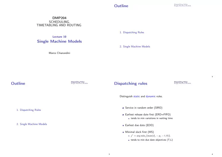
Outline Single Machine Models DMP204 SCHEDULING, TIMETABLING AND - - PowerPoint PPT Presentation

DMP204 SCHEDULING, TIMETABLING AND ROUTING

Lecture 10

Single Machine Models

Marco Chiarandini

Dispatching Rules Single Machine Models

Outline

• 1. Dispatching Rules
• 2. Single Machine Models

2 Dispatching Rules Single Machine Models

Outline

• 1. Dispatching Rules
• 2. Single Machine Models

3 Dispatching Rules Single Machine Models

Dispatching rules

Distinguish static and dynamic rules. Service in random order (SIRO) Earliest release date first (ERD=FIFO)

tends to min variations in waiting time

Earliest due date (EDD) Minimal slack first (MS)

j∗ = arg minj{max(dj − pj − t, 0)}. tends to min due date objectives (T,L)

4

Dispatching Rules Single Machine Models

(Weighted) shortest processing time first (WSPT)

j∗ = arg maxj{wj/pj}. tends to min P wjCj and max work in progress and

Loongest processing time first (LPT)

balance work load over parallel machines

Shortest setup time first (SST)

tends to min Cmax and max throughput

Least flexible job first (LFJ)

eligibility constraints

5 Dispatching Rules Single Machine Models

Critical path (CP)

first job in the CP tends to min Cmax

Largest number of successors (LNS) Shortest queue at the next operation (SQNO)

tends to min idleness of machines

6 Dispatching Rules Single Machine Models

Dispatching Rules in Scheduling

RULE DATA OBJECTIVES Rules Dependent ERD rj Variance in Throughput Times

• n Release Dates

EDD dj Maximum Lateness and Due Dates MS dj Maximum Lateness LPT pj Load Balancing over Parallel Machines Rules Dependent SPT pj Sum of Completion Times, WIP

• n Processing

WSPT pj, wj Weighted Sum of Completion Times, WIP Times CP pj, prec Makespan LNS pj, prec Makespan SIRO

• Ease of Implementation

Miscellaneous SST sjk Makespan and Throughput LFJ Mj Makespan and Throughput SQNO

• Machine Idleness

7 Dispatching Rules Single Machine Models

When dispatching rules are optimal?

8

Dispatching Rules Single Machine Models

Composite dispatching rules

Why composite rules? Example: 1 | | wjTj:

WSPT, optimal if due dates are zero EDD, optimal if due dates are loose MS, tends to minimize T

➤ The efficacy of the rules depends on instance factors

9 Dispatching Rules Single Machine Models

Instance characterization Job attributes: {weight, processing time, due date, release date} Machine attributes: {speed, num. of jobs waiting, num. of jobs eligible} Possible instance factors:

1 | | P wjTj θ1 = 1 − ¯ d Cmax (due date tightness) θ2 = dmax − dmin Cmax (due date range) 1 | sjk| P wjTj (θ1, θ2 with estimated ˆ Cmax =

n

X

j=1

pj + n¯ s) θ3 = ¯ s ¯ p (set up time severity)

10 Dispatching Rules Single Machine Models

1 | | wjTj, dynamic apparent tardiness cost (ATC) Ij(t) = wj pj exp

• −max(dj − pj − t, 0)

K ¯ p

• 1 | sjk| wjTj, dynamic apparent tardiness cost with setups (ATCS)

Ij(t, l) = wj pj exp

• −max(dj − pj − t, 0)

K1¯ p

• exp

−sjk K2¯ s

• after job l has finished.

11 Dispatching Rules Single Machine Models

Summary

Scheduling classification Solution methods Practice with general solution methods

Mathematical Programming Constraint Programming Heuristic methods

12

Dispatching Rules Single Machine Models

Outlook on Scheduling

Objectives: Look closer into scheduling models and learn: special algorithms application of general methods Cases: Single Machine Parallel Machine Permutation Flow Shop Job Shop Resource Constrained Project Scheduling

13 Dispatching Rules Single Machine Models

Outline

• 1. Dispatching Rules
• 2. Single Machine Models

14 Dispatching Rules Single Machine Models

Outlook

1 | | wjCj : weighted shortest processing time first is optimal 1 | |

j Uj : Moore’s algorithm

1 | prec| Lmax : Lawler’s algorithm, backward dynamic programming in O(n2) [Lawler, 1973] 1 | | hj(Cj) : dynamic programming in O(2n) 1 | | wjTj : local search and dynasearch 1 | rj, (prec) | Lmax : branch and bound 1 | sjk | Cmax : in the special case, Gilmore and Gomory algorithm

• ptimal in O(n2)

1 | | wjTj : column generation approaches Multicriteria

15 Dispatching Rules Single Machine Models

Summary

Single Machine Models: Cmax is sequence independent if rj = 0 and hj is monotone non decreasing in Cj then optimal schedule is nondelay and has no preemption.

16

Dispatching Rules Single Machine Models

1 | | wjCj 1 | | wjCj 1 | | wjCj

[Total weighted completion time] Theorem: The weighted shortest processing time first (WSPT) rule is

• ptimal.

Extensions to 1 | prec | wjCj in the general case strongly NP-hard chain precedences: process first chain with highest ρ-factor up to, and included, job with highest ρ-factor. polytime algorithm also for tree and sp-graph precedences

17 Dispatching Rules Single Machine Models

Extensions to 1 | rj, prmp | wjCj in the general case strongly NP-hard preemptive version of the WSPT if equal weights however, 1 | rj | wjCj is strongly NP-hard

18 Dispatching Rules Single Machine Models

1 | |

j Uj

1 | |

j Uj

1 | |

j Uj [Number of tardy jobs] [Moore, 1968] algorithm in O(n log n)

Add jobs in increasing order of due dates If inclusion of job j∗ results in this job being completed late discard the scheduled job k∗ with the longest processing time

1 | |

j wjUj is a knapsack problem hence NP-hard

19 Dispatching Rules Single Machine Models

Dynamic programming

Procedure based on divide and conquer Principle of optimality the completion of an optimal sequence of decisions must be optimal Break down the problem into stages at which the decisions take place Find a recurrence relation that takes us backward (forward) from

• ne stage to the previous (next)

(In scheduling, backward procedure feasible only if the makespan is schedule, eg, single machine problems without setups, multiple machines problems with identical processing times.)

20

Dispatching Rules Single Machine Models

1 | prec| hmax 1 | prec| hmax 1 | prec| hmax

hmax = max{h1(C1), h2(C2), . . . , hn(Cn)}, hj regular special case: 1 | prec| hmax [maximum lateness] solved by backward dynamic programming in O(n2)

[Lawler, 1978]

J set of jobs already scheduled; Jc set of jobs still to schedule; J′ ⊆ Jc set of schedulable jobs Step 1: Set J = ∅, Jc = {1, . . . , n} and J′ the set of all jobs with no successor Step 2: Select j∗ such that j∗ = arg minj∈J′{hj

• k∈Jc pk
• };

add j∗ to J; remove j∗ from Jc; update J′. Step 3: If Jc is empty then stop, otherwise go to Step 2. For 1 | | Lmax Earliest Due Date first 1|rj|Lmax is instead strongly NP-hard

21 Dispatching Rules Single Machine Models

1 | | hj(Cj) 1 | | hj(Cj) 1 | | hj(Cj)

generalization of wjTj hence strongly NP-hard (forward) dynamic programming algorithm O(2n) J set of job already scheduled; V (J) =

j∈J hj(Cj)

Step 1: Set J = ∅, V (j) = hj(pj), j = 1, . . . , n Step 2: V (J) = minj∈J

• V (J − {j}) + hj
• k∈J pk
• Step 3: If J = {1, 2, . . . , n} then V ({1, 2, . . . , n}) is optimum,
• therwise go to Step 2.

22 Dispatching Rules Single Machine Models

1 | | hj(Cj) 1 | | hj(Cj) 1 | | hj(Cj)

A lot of work done on 1 | | wjTj [single-machine total weighted tardiness] 1 | | Tj is hard in ordinary sense, hence admits a pseudo polynomial algorithm (dynamic programming in O(n4 pj)) 1 | | wjTj strongly NP-hard (reduction from 3-partition)

exact solution via branch and bound feasible up to 40 jobs [Potts and Wassenhove, Oper. Res., 1985] exact solution via time-indexed integer programming formulation used to lower bound in branch and bound solves instances of 100 jobs in 4-9 hours [Pan and Shi, Math. Progm., 2007] dynasearch: results reported for 100 jobs within a 0.005% gap from

• ptimum in less than 3 seconds [Grosso et al., Oper. Res. Lett.,

2004]

23 Dispatching Rules Single Machine Models

1 | | hj(Cj) 1 | | hj(Cj) 1 | | hj(Cj)

Local search Interchange: size n

2

• and O(|i − j|) evaluation each

first-improvement: πj, πk pπj ≤ pπk for improvements, wjTj + wkTk must decrease because jobs in πj, . . . , πk can only increase their tardiness. pπj ≥ pπk possible use of auxiliary data structure to speed up the computation best-improvement: πj, πk pπj ≤ pπk for improvements, wjTj + wkTk must decrease at least as the best interchange found so far because jobs in πj, . . . , πk can only increase their tardiness. pπj ≥ pπk possible use of auxiliary data structure to speed up the computation

Swap: size n − 1 and O(1) evaluation each Insert: size (n − 1)2 and O(|i − j|) evaluation each But possible to speed up with systematic examination by means of swaps: an interchange is equivalent to |i − j| swaps hence overall examination takes O(n2)

25

Dispatching Rules Single Machine Models

Dynasearch two interchanges δjk and δlm are independent if max{j, k} < min{l, m} or min{l, k} > max{l, m}; the dynasearch neighborhood is obtained by a series of independent interchanges; it has size 2n−1 − 1; but a best move can be found in O(n3) searched by dynamic programming; it yields in average better results than the interchange neighborhood alone.

26 Dispatching Rules Single Machine Models

state (k, π) πk is the partial sequence at state (k, π) that has min wT πk is obtained from state (i, π)

• appending job π(k) after π(i)

i = k − 1 appending job π(k) and interchanging π(i + 1) and π(k) 0 ≤ i < k − 1 F(π0) = 0; F(π1) = wπ(1)

• pπ(1) − dπ(1)

+; F(πk) = min            F(πk−1) + wπ(k)

• Cπ(k) − dπ(k)

+ , min

1≤i<k−1{F(πi) + wπ(k)

• Cπ(i) + pπ(k) − dπ(k)

+ + + k−1

j=i+2 wπ(j)

• Cπ(j) + pπ(k) − pπ(i+1) − dπ(j)

+ + +wπ(i+1)

• Cπ(k) − dπ(i+1)

+}

27 Dispatching Rules Single Machine Models

The best choice is computed by recursion in O(n3) and the optimal series of interchanges for F(πn) is found by backtrack. Local search with dynasearch neighborhood starts from an initial sequence, generated by ATC, and at each iteration applies the best dynasearch move, until no improvement is possible (that is, F(πt

n) = F(π(t−1) n

), for iteration t). Speedups:

pruning with considerations on pπ(k) and pπ(i+1) maintainig a string of late, no late jobs ht largest index s.t. π(t−1)(k) = π(t−2)(k) for k = 1, . . . , ht then F(π(t−1)

k

) = F(π(t−2)

k

) for k = 1, . . . , ht and at iter t no need to consider i < ht.

28 Dispatching Rules Single Machine Models

Dynasearch, refinements: [Grosso et al. 2004] add insertion moves to interchanges. [Ergun and Orlin 2006] show that dynasearch neighborhood can be searched in O(n2).

29