Outline DMP204 SCHEDULING, TIMETABLING AND ROUTING 1. Lagrangian - PowerPoint PPT Presentation
Outline DMP204 SCHEDULING, TIMETABLING AND ROUTING 1. Lagrangian Relaxation Lecture 12 2. Dantzig-Wolfe Decomposition Single Machine Models, Column Generation Dantzig-Wolfe Decomposition Delayed Column Generation Marco Chiarandini Slides
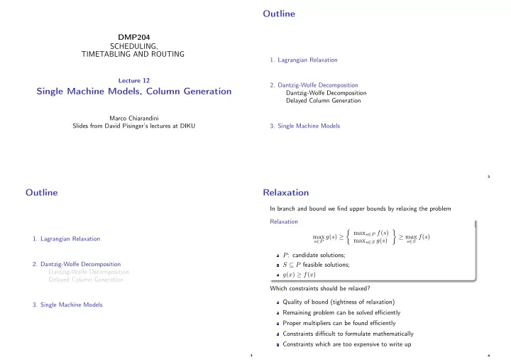
Outline DMP204 SCHEDULING, TIMETABLING AND ROUTING 1. Lagrangian Relaxation Lecture 12 2. Dantzig-Wolfe Decomposition Single Machine Models, Column Generation Dantzig-Wolfe Decomposition Delayed Column Generation Marco Chiarandini Slides from David Pisinger’s lectures at DIKU 3. Single Machine Models 2 Outline Relaxation In branch and bound we find upper bounds by relaxing the problem Relaxation � max s ∈ P f ( s ) � max s ∈ P g ( s ) ≥ ≥ max s ∈ S f ( s ) 1. Lagrangian Relaxation max s ∈ S g ( s ) P : candidate solutions; 2. Dantzig-Wolfe Decomposition S ⊆ P feasible solutions; Dantzig-Wolfe Decomposition g ( x ) ≥ f ( x ) Delayed Column Generation Which constraints should be relaxed? Quality of bound (tightness of relaxation) 3. Single Machine Models Remaining problem can be solved efficiently Proper multipliers can be found efficiently Constraints difficult to formulate mathematically Constraints which are too expensive to write up 3 4
Tightness of relaxation max cx Different relaxations s.t. Ax ≤ b Tighter LP-relaxation Dx ≤ d x ∈ Z n + Deleting constraint Best surrogate relaxation LP-relaxation: Lagrange relaxation max { cx : x ∈ conv ( Ax ≤ b, Dx ≤ d, x ∈ Z + ) } Best Lagrangian Surrogate relaxation � Lagrangian Relaxation: relaxation max z LR ( λ ) = cx − λ ( Dx − d ) Semidefinite relaxation s.t. Ax ≤ b LP relaxation x ∈ Z n + Relaxations are often used in combination. LP-relaxation: max { cx : Dx ≤ d, x ∈ conv ( Ax ≤ b, x ∈ Z + ) } 5 6 Relaxation strategies Subgradient optimization Lagrange multipliers max z = cx Which constraints should be relaxed s . t . Ax ≤ b "the complicating ones" Dx ≤ d x ∈ Z n remaining problem is polynomially solvable + Lagrange Relaxation, multipliers λ ≥ 0 (e.g. min spanning tree, assignment problem, linear programming) max z LR ( λ ) = cx − λ ( Dx − d ) remaining problem is totally unimodular s . t . Ax ≤ b (e.g. network problems) x ∈ Z n + remaining problem is NP-hard but good techniques exist Lagrange Dual Problem (e.g. knapsack) z LD = min λ ≥ 0 z LR ( λ ) constraints which cannot be expressed in MIP terms (e.g. cutting) We do not need best multipliers in B&B algorithm constraints which are too extensive to express Subgradient optimization fast method (e.g. subtour elimination in TSP) Works well due to convexity Roots in nonlinear programming, Held and Karp (1971) 7 8
Subgradient optimization, motivation Subgradient Generalization of gradients to non-differentiable functions. Definition An m -vector γ is subgradient of f ( λ ) at λ − ¯ λ if f ( λ ) ≥ f (¯ λ ) + γ ( λ − ¯ λ ) The inequality says that the hyperplane y = f (¯ λ ) + γ ( λ − ¯ λ ) is tangent to y = f ( λ ) at λ − ¯ λ and supports f ( λ ) from below Netwon-like method to minimize a Lagrange function z LR ( λ ) is function in one variable piecewise linear and convex 9 10 Intuition λ . If x ′ is an Proposition Given a choice of nonnegative multipliers ¯ Lagrange relaxation optimal solution to z LR ( λ ) then γ = d − Dx ′ max z LR ( λ ) = cx − λ ( Dx − d ) s.t. Ax ≤ b is a subgradient of z LR ( λ ) at λ = ¯ λ . x ∈ Z n + Proof We wish to prove that from the subgradient definition: Gradient in x ′ is γ = d − Dx ′ Ax ≤ b ( cx = λ ( Dx − d )) ≥ γ ( λ − ¯ cx − ¯ � � max λ ) + max λ ( Dx − d ) Ax ≤ b Subgradient Iteration where x ′ is an opt. solution to the right-most subproblem. Recursion λ k +1 = max λ k − θγ k , 0 Inserting γ we get: � � λ ) + ( cx ′ − ¯ λ ( Dx ′ − d )) ( d − Dx ′ )( λ − ¯ where θ > 0 is step-size Ax ≤ b ( cx − λ ( Dx − d )) max ≥ cx ′ − λ ( Dx ′ − d ) If γ > 0 and θ is sufficiently small z LR ( λ ) will decrease. = Small θ slow convergence Large θ unstable 11 12
Lagrange relaxation and LP For an LP-problem where we Lagrange relax all constraints Dual variables are best choice of Lagrange multipliers Lagrange relaxation and LP "relaxation" give same bound Gives a clue to solve LP-problems without Simplex Iterative algorithms Polynomial algorithms 13 14 Outline Dantzig-Wolfe Decomposition Motivation split it up into smaller pieces a large or difficult problem Applications 1. Lagrangian Relaxation Cutting Stock problems Multicommodity Flow problems 2. Dantzig-Wolfe Decomposition Facility Location problems Dantzig-Wolfe Decomposition Capacitated Multi-item Lot-sizing problem Delayed Column Generation Air-crew and Manpower Scheduling Vehicle Routing Problems 3. Single Machine Models Scheduling (current research) Two currently most promising directions for MIP: Branch-and-price Branch-and-cut 15 17
Dantzig-Wolfe Decomposition The problem is split into a master problem and a subproblem + Tighter bounds + Better control of subproblem − Model may become (very) large Delayed column generation Write up the decomposed model gradually as needed Generate a few solutions to the subproblems Solve the master problem to LP-optimality Use the dual information to find most promising solutions to the subproblem Extend the master problem with the new subproblem solutions. 18
Delayed Column Generation Delayed column generation, linear master Master problem can (and will) contain many columns To find bound, solve LP-relaxation of master Delayed column generation gradually writes up master 29
Reduced Costs � z � � � 0 B L b Simplex in matrix form = x B − 1 0 c B c L x L min { cx | Ax = b, x ≥} Simplex algorithm sets x L = 0 and x B = B − 1 b In matrix form: � 0 B invertible, hence rows linearly independent � � z � � b � A = − 1 c x 0 The objective function is obtained by multiplying and subtracting constraints by means of multipliers π (the dual variables) B = { 1 , 2 , . . . , p } basic variables p p q p p L = { 1 , 2 , . . . , q } non-basis variables (will be set to lower bound = 0) � � � � � � � � � z = c j − π i a ij + c j − π i a ij + π i b i ( B , L ) basis structure j =1 i =1 j =1 i =1 i =1 x B , x L , c B , c L , Each basic variable has cost null in the objective function B = [ A 1 , A 2 , . . . , A p ] , L = [ A p +1 , A p +2 , . . . , A p + q ] p � π = B − 1 c B c j − π i a ij = 0 = ⇒ � 0 � z � b � B L = i =1 x B − 1 c B c L 0 Reduced costs of non-basic variables: x L p � � c j − π i a ij x L = 0 x B + B − 1 Lx L = B − 1 b Bx B + Lx L = b ⇒ ⇒ x B = B − 1 b i =1 31 32
Questions Will the process terminate? Always improving objective value. Only a finite number of basis solutions. Can we repeat the same pattern? No, since the objective functions is improved. We know the best solution among existing columns. If we generate an already existing column, then we will not improve the objective. 36 Outline Scheduling 1 | prec | P w j C j Sequencing (linear ordering) variables 1. Lagrangian Relaxation n n n � � � min w j p k x kj + w j p j 2. Dantzig-Wolfe Decomposition j =1 j =1 k =1 Dantzig-Wolfe Decomposition s.t. x kj + x lk + x jl ≥ 1 j, k, l = 1 , . . . , nj � = k, k � = l Delayed Column Generation x kj + x jk = 1 ∀ j, k = 1 , . . . , n, j � = k x jk ∈ { 0 , 1 } j, k = 1 , . . . , n x jj = 0 ∀ j = 1 , . . . , n 3. Single Machine Models 38 39
Scheduling Scheduling 1 || P h j ( C j ) Time indexed variables 1 | prec | C max T − p j +1 Completion time variables n � � min h j ( t + p j ) x jt j =1 t =1 n T − p j +1 � min w j z j � s.t. x jt = 1 , for all j = 1 , . . . , n j =1 t =1 s.t. z k − z j ≥ p k for j → k ∈ A n t � � z j ≥ p j , for j = 1 , . . . , n x js ≤ 1 , for each t = 1 , . . . , T s = t − p j +1 z k − z j ≥ p k or z j − z k ≥ p j , for ( i, j ) ∈ I j =1 x jt ∈ { 0 , 1 } , for each j = 1 , . . . , n ; t = 1 , . . . , T − p j + 1 z j ∈ R , j = 1 , . . . , n + This formulation gives better bounds than the two preceding − pseudo-polynomial number of variables 40 41 Dantzig-Wolfe decomposition Dantzig-Wolfe decomposition Reformulation: Substituting X in original model getting master problem T − p j +1 n T − p j +1 n L � � min h j ( t + p j ) x jt � � � λ l x l ) min h j ( t + p j )( j =1 t =1 j =1 t =1 l =1 T − p j +1 T − p j +1 � L L s.t. x jt = 1 , for all j = 1 , . . . , n � � � λ l x l λ l n l π s.t. jt = 1 , for all j = 1 , . . . , n ⇐ = j = 1 t =1 t =1 l =1 l =1 x jt ∈ X for each j = 1 , . . . , n ; t = 1 , . . . , T − p j + 1 L � λ l = 1 , α n t � � l =1 where X = x ∈ { 0 , 1 } : x js ≤ 1 , for each t = 1 , . . . , T λ l ∈ { 0 , 1 } ⇐ = λ l ≥ 0 LP-relaxation j =1 s = t − p j +1 x l , l = 1 , . . . , L extreme points of X . matrix of X is interval matrix solve LP-relaxation by column generation on pseudo-schedules x l extreme points are integral x = � L l =1 λ l x l x ∈ { 0 , 1 } : T − p j +1 n � L � � X = ( c jt − π j ) x k l =1 λ l = 1 , reduced cost of λ k is ¯ c k = jt − α they are pseudo-schedules λ l ∈ { 0 , 1 } j =1 t =1 42 43
Recommend
More recommend
Explore More Topics
Stay informed with curated content and fresh updates.

