Outline 1) Incorporating theoretical systematics in p fits 2) - PowerPoint PPT Presentation
Is DM hidden in the p flux? Pierre Outline 1) Incorporating theoretical systematics in p fits 2) Spectral anomalies Frequentist vs Bayesian 3) A few recent examples CRAC meeting Grenoble July 5, 2019 1) Incorporating theoretical
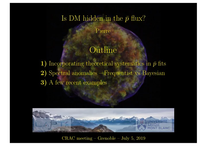
Is DM hidden in the ¯ p flux? Pierre Outline 1) Incorporating theoretical systematics in ¯ p fits 2) Spectral anomalies – Frequentist vs Bayesian 3) A few recent examples CRAC meeting – Grenoble – July 5, 2019
1) Incorporating theoretical systematics in ¯ p fits In general systematics ≡ CR + { Φ i = Φ p + Φ α } + d σ ij → ¯ p dE ¯ p Background ⌘ no DM χ 2 DM ¯ p ce CR + DM space CR space χ 2 bckg and χ 2 DM
1) Incorporating theoretical systematics in ¯ p fits In general systematics ≡ CR + { Φ i = Φ p + Φ α } + d σ ij → ¯ p dE ¯ p Background ⌘ no DM χ 2 DM ¯ p ce CR + DM space CR space ce global + DM space global space χ 2 bckg and χ 2 DM
Incorporating CR systematics in the ¯ p fit Background only vs DM hypotheses (i) Old days agnostic scan of CR parameter space to find χ 2 p , min ¯ P (¯ p | flat θ CR ) ⇒ loss of information from B/C (ii) Fit together ¯ p and B/C to get best-fit CR parameters θ CR P (¯ p + B / C | θ CR ) ⇒ not the same question Fit could be dominated by B/C and not ¯ p (iii) Fit ¯ p and incorporate a theoretical CR uncertainty matrix such as D� E C ¯ p source Φ th � � Φ th � ⌦ Φ th ↵ ⌦ Φ th ↵ = m with C B / C matrix − p p p p nm ¯ ¯ ¯ ¯ n m n C ¯ p nm = C AMS + C ¯ p source nm nm (iv) Use θ CR as nuisance parameters when fitting ¯ p data χ 2 = χ 2 CR ≡ ( θ p − ¯ pq ( θ q − ¯ � χ 2 θ p ) C CR p + θ q ) ¯ How is C CR pq defined? If C CR ≡ C B / C ⇒ back to (iii) Bayesian with P ( θ CR | ¯ p ) = L (¯ p | θ CR ) × Π ( θ CR )
2) Spectral anomalies – Frequentist vs Bayesian (a) Model M i is wright or wrong depending on its reduced χ 2 per d.o.f. Frequentist approach – models M 1 and M 2 are both true Maximum likelihood method if M 1 ⊂ M 2 (b) Generate Mock data sets with best-fit model M 1 , fit them and look for the Monte Carlo distribution of ∆ χ 2 = χ 2 1 − χ 2 2 . Conclude from P ( ∆ χ 2 | M 1 ) Mock data to be generated – lengthy procedure Frequentist approach – may be the best one (c) Use the Akaike information criterion (AIC) and compute the di ff erence ∆ AIC = AIC 2 − AIC 1 . AIC = 2 p − 2 ln L max with p parameters AIC cor = AIC + 2 p 2 + 2 p N − p − 1 with N data points In our example, N is large and ∆ AIC = 4 − ∆ χ 2 P ( M 1 ) P ( M 2 ) = e ∆ AIC / 2 In Cuoco et al. (2019) P (no DM) /P (DM) = 1 . 3 × 10 − 2
(d) Bayesian approach in the spirit of method iv with nuisance parameters. In this example θ 1 = { θ CR } while θ 2 = { θ CR , h σ ann v i , m χ } . Compute the probability P (¯ p | M i ) and use Bayes factor K . p, M 1 ) = L ( ¯ p | θ 1 , M 1 ) Π ( θ 1 | M 1 ) P ( θ 1 | ¯ P (¯ p | M 1 ) Z P (¯ p | M 1 ) = L ( ¯ p | θ 1 , M 1 ) Π ( θ 1 | M 1 ) d θ 1 P ( M 2 | ¯ p ) ⇢ K ⌘ P (¯ p | M 2 ) � ⇢ P ( M 2 ) � p ) = P ( M 1 ) ' 1 P ( M 1 | ¯ P (¯ p | M 1 ) Je ff reys’ scale (e) Use the Schwarz/Bayes information criterion (SBIC) and compute the di ff erence ∆ SBIC = SBIC 2 � SBIC 1 . SBIC = p ln( N ) � 2 ln L max with p parameters In our example, N = 158 and ∆ SBIC = 10 . 1 � ∆ χ 2 P ( M 1 | ¯ p ) p ) = e ∆ SBIC / 2 P ( M 2 | ¯ In Cuoco et al. (2019) P (no DM) /P (DM) = 0 . 28 (no comment)
(d) Bayesian approach in the spirit of method iv with nuisance parameters. In this example θ 1 = { θ CR } while θ 2 = { θ CR , h σ ann v i , m χ } . Compute the probability P (¯ p | M i ) and use Bayes factor K . p, M 1 ) = L ( ¯ p | θ 1 , M 1 ) Π ( θ 1 | M 1 ) P ( θ 1 | ¯ P (¯ p | M 1 ) Z P (¯ p | M 1 ) = L ( ¯ p | θ 1 , M 1 ) Π ( θ 1 | M 1 ) d θ 1 P ( M 2 | ¯ p ) ⇢ K ⌘ P (¯ p | M 2 ) � ⇢ P ( M 2 ) � p ) = P ( M 1 ) ' 1 P ( M 1 | ¯ P (¯ p | M 1 ) (e) Use the Schwarz/Bayes information criterion (SBIC) and compute the di ff erence ∆ SBIC = SBIC 2 � SBIC 1 . SBIC = p ln( N ) � 2 ln L max with p parameters In our example, N = 158 and ∆ SBIC = 10 . 1 � ∆ χ 2 P ( M 1 | ¯ p ) p ) = e ∆ SBIC / 2 P ( M 2 | ¯ In Cuoco et al. (2019) P (no DM) /P (DM) = 0 . 28 (no comment)
3) A few recent examples A. Cuoco et al, Phys. Rev. D99 (2019) 103014 Method (ii) used to look for DM with P ( p + α + ¯ p/p | θ CR )
3) A few recent examples A. Cuoco et al, Phys. Rev. D99 (2019) 103014 Method (ii) used to look for DM with P ( p + α + ¯ p/p | θ CR )
3) A few recent examples A. Cuoco et al, Phys. Rev. D99 (2019) 103014 ⇒ Method (e) , i.e., Schwarz/Bayes information criterion, yields P (no DM | data) = e ∆ SBIC / 2 = 0 . 28 P (DM | data) Method (ii) used to look for DM with P ( p + α + ¯ p/p | θ CR )
Mixed methods (ii) + (iii) used to look for DM A. Reinert & M.W. Winkler, JCAP 1801 (2018) 055 + Σ B / C source Uncertainties on XS treated with Σ ¯ p source nm nm p + B / C + AMS / PAMELA | θ CR + φ F P (¯ p ) ¯ Method (b) used Mock data ⇒ ∆ χ 2 & P ( ∆ χ 2 | M 1 ) P (no DM | data) = e ∆ SBIC / 2 = 13 . 5 & 42 . 5 ⇒ P (DM | data) Method (e) , i.e., Schwarz/Bayes information criterion, yields ∆ SBIC = 2 ln( N ) − 2 ∆ ln L max = 9 . 9 − ∆ χ 2 DM is 7.4% (¯ bb) and 2.4% (WW) as probable as no DM!
Recommend
More recommend
Explore More Topics
Stay informed with curated content and fresh updates.
