Outline Interactions with grouping factors Mixed models in R using - PowerPoint PPT Presentation

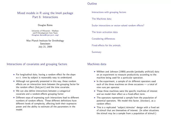
Outline Interactions with grouping factors Mixed models in R using the lme4 package Part 6: Interactions The Machines data Douglas Bates Scalar interactions or vector-valued random effects? University of Wisconsin - Madison The brain activation data and R Development Core Team <Douglas.Bates@R-project.org> Considering differences Max Planck Institute for Ornithology Seewiesen Fixed-effects for the animals July 21, 2009 Summary Interactions of covariates and grouping factors Machines data ◮ Milliken and Johnson (1989) provide (probably artificial) data ◮ For longitudinal data, having a random effect for the slope on an experiment to measure productivity according to the w.r.t. time by subject is reasonably easy to understand. machine being used for a particular operation. ◮ Although not generally presented in this way, these random ◮ In the experiment, a sample of six different operators used effects are an interaction term between the grouping factor for each of the three machines on three occasions — a total of the random effect ( Subject ) and the time covariate. nine runs per operator. ◮ We can also define interactions between a categorical ◮ These three machines were the specific machines of interest covariate and a random-effects grouping factor. and we model their effect as a fixed-effect term. ◮ Different ways of expressing such interactions lead to different ◮ The operators represented a sample from the population of numbers of random effects. These different definitions have potential operators. We model this factor, ( Worker ), as a different levels of complexity, affecting both their expressive random effect. power and the ability to estimate all the parameters in the ◮ This is a replicated “subject/stimulus” design with a fixed set model. of stimuli that are themselves of interest. (In other situations the stimuli may be a sample from a population of stimuli.)

Machines data plot Comments on the data plot A B C ● ◮ There are obvious differences between the scores on different ●● 3 ● machines. ◮ It seems likely that Worker will be a significant random effect, ● ● 5 ● especially when considering the low variation within replicates. ● ● ◮ There also appears to be a significant Worker:Machine 1 ● Worker interaction. Worker 6 has a very different pattern w.r.t. ● ● 4 machines than do the others. ● ◮ We can approach the interaction in one of two ways: define ● 2 ● ● simple, scalar random effects for Worker and for the Worker:Machine interaction or define vector-valued random ● 6 ● ● effects for Worker 45 50 55 60 65 70 Quality and productivity score Random effects for subject and subject:stimulus Characteristics of the scalar interaction model ◮ The model incorporates simple, scalar random effects for Linear mixed model fit by REML Formula: score ~ Machine + (1 | Worker) + (1 | Worker:Machine) Worker and for the Worker:Machine interaction. Data: Machines ◮ These two scalar random-effects terms have q 1 = q 2 = 1 so AIC BIC logLik deviance REMLdev 227.7 239.6 -107.8 225.5 215.7 they contribute n 1 = 6 and n 2 = 18 random effects for a total Random effects: of q = 24 . There are 2 variance-component parameters. Groups Name Variance Std.Dev. ◮ The random effects allow for an overall shift in level for each Worker:Machine (Intercept) 13.90946 3.72954 Worker (Intercept) 22.85849 4.78105 worker and a separate shift for each combination of worker Residual 0.92463 0.96158 and machine. The unconditional distributions of these random Number of obs: 54, groups: Worker:Machine, 18; Worker, 6 effects are independent. The unconditional variances of the Fixed effects: interaction random effects are constant. Estimate Std. Error t value (Intercept) 52.356 2.486 21.063 ◮ The main restriction in this model is the assumption of MachineB 7.967 2.177 3.660 constant variance and independence of the interaction random MachineC 13.917 2.177 6.393 effects.

Model matrix Z T for the scalar interaction model Vector-valued random effects by subject Linear mixed model fit by REML Formula: score ~ Machine + (0 + Machine | Worker) Data: Machines 5 AIC BIC logLik deviance REMLdev 228.3 248.2 -104.2 216.6 208.3 10 Random effects: Row Groups Name Variance Std.Dev. Corr 15 Worker MachineA 16.64097 4.07933 MachineB 74.39556 8.62529 0.803 20 MachineC 19.26756 4.38948 0.623 0.771 Residual 0.92463 0.96158 10 20 30 40 50 Number of obs: 54, groups: Worker, 6 Column Fixed effects: Estimate Std. Error t value (Intercept) 52.356 1.681 31.150 ◮ Because we know these are scalar random effects we can MachineB 7.967 2.421 3.291 recognize the pattern of a balanced, nested, two-factor design, MachineC 13.917 1.540 9.037 similar to that of the model for the Pastes data. Characteristics of the vector-valued r.e. model Comparing the model fits ◮ Although not obvious from the specifications, these model fits are nested. If the variance-covariance matrix for the 5 vector-valued random effects has a special form, called 10 compound symmetry , the model reduces to model fm1 . 15 ◮ The p-value of 6.5% may or may not be significant. 10 20 30 40 50 > fm2M <- update(fm2, REML = FALSE) > fm1M <- update(fm1, REML = FALSE) > anova(fm2M, fm1M) ◮ We use the specification (0 + Machine|Worker) to force an Data: Machines “indicator” parameterization of the random effects. Models: ◮ In this image the 1’s are black. The gray positions are fm1M: score ~ Machine + (1 | Worker) + (1 | Worker:Machine) fm2M: score ~ Machine + (0 + Machine | Worker) non-systematic zeros (initially zero but can become nonzero). Df AIC BIC logLik Chisq Chi Df Pr(>Chisq) ◮ Here k = 1 , q 1 = 3 and n 1 = 6 so we have q = 18 random fm1M 6 237.27 249.20 -112.64 effects but q 1 ( q 1 + 1) / 2 = 6 variance-component parameters fm2M 10 236.42 256.31 -108.21 8.8516 4 0.06492 to estimate.

Model comparisons eliminating the unusual combination Machines data after eliminating the unusual combination A B C ● ◮ In a case like this we may want to check if a single, unusual ● ●● 3 combination ( Worker 6 using Machine “B”) causes the more complex model to appear necessary. We eliminate that ● 5 ● ● unusual combination. ● ● > Machines1 <- subset(Machines, !(Worker == "6" & Machine == 1 ● Worker + "B")) > xtabs(~Machine + Worker, Machines1) ● ● 4 ● Worker ● 2 ● ● Machine 1 2 3 4 5 6 A 3 3 3 3 3 3 ● B 3 3 3 3 3 0 6 ● ● C 3 3 3 3 3 3 45 50 55 60 65 70 Quality and productivity score Model comparisons without the unusual combination Trade-offs when defining interactions ◮ It is important to realize that estimating scale parameters (i.e. variances and covariances) is considerably more difficult than estimating location parameters (i.e. means or fixed-effects > fm1aM <- lmer(score ~ Machine + (1 | Worker) + (1 | coefficients). + Worker:Machine), Machines1, REML = FALSE) > fm2aM <- lmer(score ~ Machine + (0 + Machine | Worker), ◮ A vector-valued random effect term having q i random effects + Machines1, REML = FALSE) per level of the grouping factor requires q i ( q i + 1) / 2 > anova(fm2aM, fm1aM) variance-covariance parameters to be estimated. A simple, Data: Machines1 scalar random effect for the interaction of a “random-effects” Models: factor and a “fixed-effects” factor requires only 1 additional fm1aM: score ~ Machine + (1 | Worker) + (1 | Worker:Machine) variance-covariance parameter. fm2aM: score ~ Machine + (0 + Machine | Worker) Df AIC BIC logLik Chisq Chi Df Pr(>Chisq) ◮ Especially when the “fixed-effects” factor has a moderate to fm1aM 6 208.554 220.145 -98.277 large number of levels, the trade-off in model complexity fm2aM 10 208.289 227.607 -94.144 8.2655 4 0.08232 argues against the vector-valued approach. ◮ One of the major sources of difficulty in using the lme4 package is the tendency to overspecify the number of random effects per level of a grouping factor.