Out-of-equilibrium field theories coupled to strong external sources - PowerPoint PPT Presentation
Out-of-equilibrium field theories coupled to strong external sources Kyoto University, December 2013 Franois Gelis IPhT, Saclay Outline 1 Preamble : classical statistical method in Quantum Mechanics 2 QFT with strong sources, Inclusive
Out-of-equilibrium field theories coupled to strong external sources Kyoto University, December 2013 François Gelis IPhT, Saclay
Outline 1 Preamble : classical statistical method in Quantum Mechanics 2 QFT with strong sources, Inclusive observables at LO and NLO 3 Instabilities and resummation 4 Example : Schwinger mechanism
Quantum Mechanics
Classical phase-space formulation of Quantum Mechanics • Consider the von Neumann equation for the density operator : �� � ∂ � ρ τ ∂τ = i ¯ h H, � ρ τ (**) • Introduce the Wigner transforms : � d s e i p · s � � � � x + s � x − s �� W τ ( x , p ) ≡ ρ τ 2 2 � d s e i p · s � � � � x + s � x − s �� H ( x , p ) ≡ H (classical Hamiltonian) 2 2 (**) is equivalent to : � i ¯ �� � ← ∂W τ H ( x , p ) 2 h → ← → = ∂ x − W τ ( x , p ) h sin ∂ p ∂ x ∂ p ∂τ i ¯ 2 � � h 2 ) = H , W τ + O ( ¯ � �� � Poisson bracket François Gelis Field theories with strong sources 1/39 Kyoto, December 2013
Classical statistical method in Quantum Mechanics h 2 ) corrections • Quantum effects in the time evolution are O ( ¯ (i.e. they appear at NNLO and beyond) • O ( ¯ h ) (NLO) contributions can only come from the initial state Uncertainty principle : ∆ x · ∆ p ≥ ¯ h The initial Wigner distribution W τ = 0 ( x , p ) must have a support of area at least ¯ (minimal area realized by coherent states) h • All the O ( ¯ h ) effects can be accounted for by a Gaussian initial distribution W τ = 0 ( x , p ) Classical statistical method • Sample by a Monte-Carlo the Gaussian distribution that approximates the initial distribution W τ = 0 ( x , p ) • For each initial ( x , p ) , solve the classical equation of motion up to the time of interest François Gelis Field theories with strong sources 2/39 Kyoto, December 2013
Decoherence and micro-canonical equilibration P Q • For non-harmonic oscillators, the oscillation frequency depends on the initial condition François Gelis Field theories with strong sources 3/39 Kyoto, December 2013
Decoherence and micro-canonical equilibration P Q • For non-harmonic oscillators, the oscillation frequency depends on the initial condition • Because of QM, the initial ensemble is a set of width � ¯ h François Gelis Field theories with strong sources 3/39 Kyoto, December 2013
Decoherence and micro-canonical equilibration P Q • For non-harmonic oscillators, the oscillation frequency depends on the initial condition • Because of QM, the initial ensemble is a set of width � ¯ h • This ensemble of initial configurations spreads in time François Gelis Field theories with strong sources 3/39 Kyoto, December 2013
Decoherence and micro-canonical equilibration P Q • For non-harmonic oscillators, the oscillation frequency depends on the initial condition • Because of QM, the initial ensemble is a set of width � ¯ h • This ensemble of initial configurations spreads in time François Gelis Field theories with strong sources 3/39 Kyoto, December 2013
Decoherence and micro-canonical equilibration P Q • For non-harmonic oscillators, the oscillation frequency depends on the initial condition • Because of QM, the initial ensemble is a set of width � ¯ h • This ensemble of initial configurations spreads in time • At large times, the ensemble fills densely all the region allowed by energy conservation ⇒ microcanonical equilibrium François Gelis Field theories with strong sources 3/39 Kyoto, December 2013
Quantum Field Theory w/ Strong Sources
Typical situation 1 2 ( ∂ µ φ )( ∂ µ φ ) − V ( φ ) + Jφ • In general, the source J is space and time dependent • The system starts at t = − ∞ from a known initial state (example: vacuum state) • The source may be turned off at some point, and the system evolves by itself afterwards Strong source : J ∼ inverse coupling • Non-perturbative can we expand in powers of the coupling? ⇒ = • Spectrum of produced particles? • After the sources are switched off : how does the system equilibrate? François Gelis Field theories with strong sources 4/39 Kyoto, December 2013
Example I : Schwinger mechanism • Consider a constant and uniform electrical field � E ext • Perturbatively, energy conservation prevents the production of e + e − pairs • Pairs can be produced via a vacuum instability • Rate : exp (− πm 2 /eE ) (non analytic in the coupling e ) • In Quantum Field Theory, can be obtained at one loop (but one must use the propagator dressed by the external field) François Gelis Field theories with strong sources 5/39 Kyoto, December 2013
Example II : Nucleus-Nucleus collisions at high energy ? L = − 1 4 F µν F µν + ( J µ 1 + J µ ) A µ 2 � �� � J µ • Given the sources J 1,2 in each projectile, how do we calculate observables? Is there some kind of perturbative expansion? • Loop corrections, factorization? • Thermalization? François Gelis Field theories with strong sources 6/39 Kyoto, December 2013
Strong source regime • Weak sources : perturbative treatment François Gelis Field theories with strong sources 7/39 Kyoto, December 2013
Strong source regime • Weak sources : perturbative treatment • Strong sources : non-perturbative (when J ∼ 1/g ) François Gelis Field theories with strong sources 7/39 Kyoto, December 2013
Power counting François Gelis Field theories with strong sources 8/39 Kyoto, December 2013
Power counting Order of connected subdiagram when J ∼ g − 1 : 1 g 2 g # produced gluons g 2 ( # loops ) François Gelis Field theories with strong sources 8/39 Kyoto, December 2013
Power counting • Example : single particle spectrum : � � dN 1 p = 1 c 0 + c 1 g 2 + c 2 g 4 + · · · d 3 � g 2 • The coefficients c 0 , c 1 , · · · are themselves series that resum all orders in ( gJ ) n . For instance, ∞ � c 0,n ( gJ ) n c 0 = n = 0 • We want to calculate at least the entire c 0 /g 2 contribution, and a subset of the higher order terms François Gelis Field theories with strong sources 9/39 Kyoto, December 2013
Inclusive observables • Inclusive observables do not veto any final state Example: moments of the transition probabilities : � ∞ dN 1 � 1 2 � � � �� � � p ∼ ( n + 1 ) dΦ 1 · · · dΦ n pp 1 · · · p n out � 0 in � � d 3 � ( n + 1 )! � �� � � � n = 0 n part. phase-space (single inclusive particle distribution) Equivalent definition : � � � � dN 1 � a † � 0 in p ∼ 0 in out ( p ) a out ( p ) d 3 � (completeness of the out-states) François Gelis Field theories with strong sources 10/39 Kyoto, December 2013
Bookkeeping • Start with transition amplitudes : sources → particles François Gelis Field theories with strong sources 11/39 Kyoto, December 2013
Bookkeeping • Start with transition amplitudes : sources → particles • Consider squared amplitudes (including interferences) François Gelis Field theories with strong sources 11/39 Kyoto, December 2013
Bookkeeping • Start with transition amplitudes : sources → particles • Consider squared amplitudes (including interferences) • See them as cuts through vacuum diagrams Cut propagator ∼ δ ( p 2 ) François Gelis Field theories with strong sources 11/39 Kyoto, December 2013
Bookkeeping • Start with transition amplitudes : sources → particles • Consider squared amplitudes (including interferences) • See them as cuts through vacuum diagrams Cut propagator ∼ δ ( p 2 ) Weight each cut by z ( p ) generating functional → � � � 1 2 � � �� � � F [ z ] ≡ dΦ 1 · · · dΦ n z ( p 1 ) · · · z ( p n ) p 1 · · · p n out � 0 in � � n ! � � n François Gelis Field theories with strong sources 11/39 Kyoto, December 2013
Generating functional • Observables are given by derivatives of F [ z ] , e.g. � � dN 1 p = δF [ z ] � � d 3 � δz ( p ) z = 1 (inclusive observables are derivatives at the point z = 1 ) unitarity implies F [ 1 ] = 1 Exact formula for the first derivative : � δ log F [ z ] d 4 xd 4 y e ip · ( x − y ) � x � y � � = A + ( x ) A − ( y ) + G +− ( x, y ) δz ( p ) where A ± and G +− are connected 1- and 2-point functions in the Schwinger-Keldysh formalism, with cut propagators weighted by z ( p ) François Gelis Field theories with strong sources 12/39 Kyoto, December 2013
Schwinger-Keldysh formalism • Set of Feynman rules to compute directly transition probabilities (i.e. AA ∗ ) • This can be achieved as follows : • A vertex is − ig on one side of the cut, and + ig on the other side • There are four propagators, depending on the location w.r.t. the cut of the vertices they connect : ++ ( p ) = i/ ( p 2 − m 2 + iǫ ) G 0 ( standard Feynman propagator ) −− ( p ) = − i/ ( p 2 − m 2 − iǫ ) G 0 ( complex conjugate of G 0 ++ ( p )) +− ( p ) = 2π z ( p ) θ (− p 0 ) δ ( p 2 − m 2 ) G 0 • At each vertex of a given diagram, sum over the types + and − ( 2 n terms for a diagram with n vertices) François Gelis Field theories with strong sources 13/39 Kyoto, December 2013
Inclusive Observables at Leading Order
Recommend
More recommend
Explore More Topics
Stay informed with curated content and fresh updates.
