Optimization and Simulation Optimization Michel Bierlaire - PowerPoint PPT Presentation
Optimization and Simulation Optimization Michel Bierlaire Transport and Mobility Laboratory School of Architecture, Civil and Environmental Engineering Ecole Polytechnique F ed erale de Lausanne M. Bierlaire (TRANSP-OR ENAC EPFL)
Greedy heuristics Example x ∈ R 2 − 3 x 1 − 13 x 2 min subject to 2 x 1 + 9 x 2 ≤ 40 11 x 1 − 8 x 2 ≤ 82 x 1 , x 2 ≥ 0 x 1 , x 2 ∈ N M. Bierlaire (TRANSP-OR ENAC EPFL) Optimization and Simulation 36 / 108
Greedy heuristics Relaxation: feasible set 5 4 3 2 1 0 0 1 2 3 4 5 6 7 8 9 10 M. Bierlaire (TRANSP-OR ENAC EPFL) Optimization and Simulation 37 / 108
Greedy heuristics Optimal solution of the relaxation 5 4 3 2 1 Opt. solution relaxation (9 . 2 , 2 . 4) 0 0 1 2 3 4 5 6 7 8 9 10 M. Bierlaire (TRANSP-OR ENAC EPFL) Optimization and Simulation 38 / 108
Greedy heuristics Integrality constraints 5 4 3 2 1 Opt. solution relaxation (9 . 2 , 2 . 4) 0 0 1 2 3 4 5 6 7 8 9 10 M. Bierlaire (TRANSP-OR ENAC EPFL) Optimization and Simulation 39 / 108
Greedy heuristics Infeasible neighbors 5 Infeasible neighbors 4 3 2 1 Opt. solution relaxation (9 . 2 , 2 . 4) 0 0 1 2 3 4 5 6 7 8 9 10 M. Bierlaire (TRANSP-OR ENAC EPFL) Optimization and Simulation 40 / 108
Greedy heuristics Solution of the integer optimization problem 5 Infeasible neighbors 4 3 2 Optimal solution (integer) 1 Opt. solution relaxation (9 . 2 , 2 . 4) 0 0 1 2 3 4 5 6 7 8 9 10 M. Bierlaire (TRANSP-OR ENAC EPFL) Optimization and Simulation 41 / 108
Greedy heuristics Issues There are 2 n different ways to round. Which one to choose? Rounding may generate an infeasible solution. The rounded solution may be far from the optimal solution. M. Bierlaire (TRANSP-OR ENAC EPFL) Optimization and Simulation 42 / 108
Neighborhood and local search Outline Introduction 1 Classical optimization problems 2 Greedy heuristics 3 Neighborhood and local search 4 Diversification 5 Variable Neighborhood Search Simulated annealing Comments M. Bierlaire (TRANSP-OR ENAC EPFL) Optimization and Simulation 43 / 108
Neighborhood and local search Neighborhood and local search Concept The feasible set is too large. At each iteration, restrict the optimization problem to a small feasible subset. Ideally, the small subset can be enumerated. Typically, it consists of solutions obtained from simple modifications of the current solution. The small subset is called a neighborhood . M. Bierlaire (TRANSP-OR ENAC EPFL) Optimization and Simulation 44 / 108
Neighborhood and local search Integer optimization: neighborhood Consider the current iterate x ∈ Z n . For each k = 1 , . . . , n , define 2 neighbors by increasing and decreasing the value of x k by one unit. The neighbors y k + and y k − are defined as y k + = y k − y k + y k + = x i , ∀ i � = k , = x k + 1 , = x k − 1 . i i k k Example y 2+ = (3 , 6 , 2 , 8) y 2 − = (3 , 4 , 2 , 8) x = (3 , 5 , 2 , 8) M. Bierlaire (TRANSP-OR ENAC EPFL) Optimization and Simulation 45 / 108
Neighborhood and local search Integer optimization: neighborhood x M. Bierlaire (TRANSP-OR ENAC EPFL) Optimization and Simulation 46 / 108
Neighborhood and local search Integer optimization: neighborhood The concept of neighborhood is fairly general. It must be defined based on the structure of the problem. Creativity is required here. x M. Bierlaire (TRANSP-OR ENAC EPFL) Optimization and Simulation 47 / 108
Neighborhood and local search Local search Consider the integer optimization problem x ∈ Z n f ( x ) min subject to x ∈ F . Consider the neighborhood structure V ( x ), where V ( x ) is the set of neighbors of x . At each iteration k , consider the neighbors in V ( x k ) one at a time. For each y ∈ V ( x k ), if f ( y ) < f ( x k ), then x k +1 = y and proceed to the next iteration. If f ( y ) ≥ f ( x k ), ∀ y ∈ V ( x k ), x k is a local minimum. Stop. M. Bierlaire (TRANSP-OR ENAC EPFL) Optimization and Simulation 48 / 108
Neighborhood and local search Local search: example x ∈ R 2 − 3 x 1 − 13 x 2 min subject to 2 x 1 + 9 x 2 ≤ 40 11 x 1 − 8 x 2 ≤ 82 x 1 , x 2 ∈ N M. Bierlaire (TRANSP-OR ENAC EPFL) Optimization and Simulation 49 / 108
Neighborhood and local search Local search: example 5 4 3 2 1 0 0 1 2 3 4 5 6 7 8 9 10 M. Bierlaire (TRANSP-OR ENAC EPFL) Optimization and Simulation 50 / 108
Neighborhood and local search Local search: example x 0 = (6 , 0) - Neighborhood: E - N - O - S 5 4 3 2 1 0 0 1 2 3 4 5 6 7 8 9 10 M. Bierlaire (TRANSP-OR ENAC EPFL) Optimization and Simulation 51 / 108
Neighborhood and local search Local search: example x 0 = (0 , 3) - Neighborhood: E - N - O - S 5 4 3 2 1 0 0 1 2 3 4 5 6 7 8 9 10 M. Bierlaire (TRANSP-OR ENAC EPFL) Optimization and Simulation 52 / 108
Neighborhood and local search Local search: example x 0 = (6 , 0) - Neighborhood : N - O - S - E 5 4 3 2 1 0 0 1 2 3 4 5 6 7 8 9 10 M. Bierlaire (TRANSP-OR ENAC EPFL) Optimization and Simulation 53 / 108
Neighborhood and local search Local search: comments The algorithm stops at a local minimum, that is a solution better than all its neighbors. The outcome depends on the starting point and the structure of the neighborhood. The neighborhood must be sufficiently large to increase the chances of improvement, and sufficiently small to avoid a lengthy enumeration. Example of a neighborhood too small: one neighbor at the west. Example of a neighborhood too large: each feasible point is in the neighborhood. It is good practice to use symmetric neighborhoods: y ∈ V ( x ) ⇐ ⇒ x ∈ V ( y ) . M. Bierlaire (TRANSP-OR ENAC EPFL) Optimization and Simulation 54 / 108
Neighborhood and local search The knapsack problem x ∈{ 0 , 1 } n u T x max subject to w T x ≤ W . M. Bierlaire (TRANSP-OR ENAC EPFL) Optimization and Simulation 55 / 108
Neighborhood and local search The knapsack problem: neighborhood Current solution: for each item i , x i = 0 or x i = 1. Neighbor solution: select an item j , and change the decision: x j ← 1 − x j . Warning: check feasibility. Generalization: neighborhood of size k : select k items, and change the decision for them (checking feasibility). M. Bierlaire (TRANSP-OR ENAC EPFL) Optimization and Simulation 56 / 108
Neighborhood and local search The knapsack problem: neighborhood A neighborhood of size k modifies k variables. Number of neighbors: n ! k !( n − k )! k = 1: n neighbors. k = n : 1 neighbor. Example : W = 300. i 1 2 3 4 5 6 7 8 9 10 11 12 U 80 31 48 17 27 84 34 39 46 58 23 67 W 84 27 47 22 21 96 42 46 54 53 32 78 First solution: empty sack. M. Bierlaire (TRANSP-OR ENAC EPFL) Optimization and Simulation 57 / 108
Neighborhood and local search The knapsack problem: local search w T x c u T x c u T x ∗ 1 2 3 4 5 6 7 8 9 10 11 12 k 0 0 0 0 0 0 0 0 0 0 0 0 0 0 0 0 1 1 0 0 0 0 0 0 0 0 0 0 0 84 80 0 M. Bierlaire (TRANSP-OR ENAC EPFL) Optimization and Simulation 58 / 108
Neighborhood and local search The knapsack problem: local search w T x c u T x c u T x ∗ k 1 2 3 4 5 6 7 8 9 10 11 12 1 1 0 0 0 0 0 0 0 0 0 0 0 84 80 0 0 0 0 0 0 0 0 0 0 0 0 0 0 80 2 1 1 0 0 0 0 0 0 0 0 0 0 111 111 80 M. Bierlaire (TRANSP-OR ENAC EPFL) Optimization and Simulation 59 / 108
Neighborhood and local search The knapsack problem: local search w T x c u T x c u T x ∗ k 1 2 3 4 5 6 7 8 9 10 11 12 2 1 1 0 0 0 0 0 0 0 0 0 0 111 111 0 1 0 0 0 0 0 0 0 0 0 0 27 31 111 1 0 0 0 0 0 0 0 0 0 0 0 84 80 111 3 1 1 1 0 0 0 0 0 0 0 0 0 158 159 111 M. Bierlaire (TRANSP-OR ENAC EPFL) Optimization and Simulation 60 / 108
Neighborhood and local search The knapsack problem: local search w T x c u T x c u T x ∗ k 1 2 3 4 5 6 7 8 9 10 11 12 3 1 1 1 0 0 0 0 0 0 0 0 0 158 159 0 1 1 0 0 0 0 0 0 0 0 0 74 79 159 1 0 1 0 0 0 0 0 0 0 0 0 131 128 159 1 1 0 0 0 0 0 0 0 0 0 0 111 111 159 4 1 1 1 1 0 0 0 0 0 0 0 0 180 176 159 M. Bierlaire (TRANSP-OR ENAC EPFL) Optimization and Simulation 61 / 108
Neighborhood and local search The knapsack problem: local search w T x c u T x c u T x ∗ 1 2 3 4 5 6 7 8 9 10 11 12 k 4 1 1 1 1 0 0 0 0 0 0 0 0 180 176 0 1 1 1 0 0 0 0 0 0 0 0 96 96 176 1 0 1 1 0 0 0 0 0 0 0 0 153 145 176 1 1 0 1 0 0 0 0 0 0 0 0 133 128 176 1 1 1 0 0 0 0 0 0 0 0 0 158 159 176 5 1 1 1 1 1 0 0 0 0 0 0 0 201 203 176 M. Bierlaire (TRANSP-OR ENAC EPFL) Optimization and Simulation 62 / 108
Neighborhood and local search The knapsack problem: local search w T x c u T x c u T x ∗ k 1 2 3 4 5 6 7 8 9 10 11 12 5 1 1 1 1 1 0 0 0 0 0 0 0 201 203 0 1 1 1 1 0 0 0 0 0 0 0 117 123 203 1 0 1 1 1 0 0 0 0 0 0 0 174 172 203 1 1 0 1 1 0 0 0 0 0 0 0 154 155 203 1 1 1 0 1 0 0 0 0 0 0 0 179 186 203 1 1 1 1 0 0 0 0 0 0 0 0 180 176 203 6 1 1 1 1 1 1 0 0 0 0 0 0 297 287 203 M. Bierlaire (TRANSP-OR ENAC EPFL) Optimization and Simulation 63 / 108
Neighborhood and local search The knapsack problem: local search w T x c u T x c u T x ∗ k 1 2 3 4 5 6 7 8 9 10 11 12 6 1 1 1 1 1 1 0 0 0 0 0 0 297 287 0 1 1 1 1 1 0 0 0 0 0 0 213 207 287 1 0 1 1 1 1 0 0 0 0 0 0 270 256 287 1 1 0 1 1 1 0 0 0 0 0 0 250 239 287 1 1 1 0 1 1 0 0 0 0 0 0 275 270 287 1 1 1 1 0 1 0 0 0 0 0 0 276 260 287 1 1 1 1 1 0 0 0 0 0 0 0 201 203 287 1 1 1 1 1 1 1 0 0 0 0 0 339 321 287 1 1 1 1 1 1 0 1 0 0 0 0 343 326 287 1 1 1 1 1 1 0 0 1 0 0 0 351 333 287 1 1 1 1 1 1 0 0 0 1 0 0 350 345 287 1 1 1 1 1 1 0 0 0 0 1 0 329 310 287 1 1 1 1 1 1 0 0 0 0 0 1 375 354 287 M. Bierlaire (TRANSP-OR ENAC EPFL) Optimization and Simulation 64 / 108
Neighborhood and local search TSP: 12 cities 10 9 8 11 7 H 6 5 2 1 4 3 M. Bierlaire (TRANSP-OR ENAC EPFL) Optimization and Simulation 65 / 108
Neighborhood and local search Initial solution from greedy algorithm 10 9 8 11 7 H 6 5 2 1 4 3 M. Bierlaire (TRANSP-OR ENAC EPFL) Optimization and Simulation 66 / 108
Neighborhood and local search Initial solution from greedy algorithm 10 9 8 11 7 H 6 5 2 1 4 3 M. Bierlaire (TRANSP-OR ENAC EPFL) Optimization and Simulation 67 / 108
Neighborhood and local search Initial solution from greedy algorithm 10 9 8 11 7 H 6 5 2 1 4 3 M. Bierlaire (TRANSP-OR ENAC EPFL) Optimization and Simulation 68 / 108
Neighborhood and local search Initial solution from greedy algorithm 10 9 8 11 7 H 6 5 2 1 4 3 M. Bierlaire (TRANSP-OR ENAC EPFL) Optimization and Simulation 69 / 108
Neighborhood and local search Initial solution from greedy algorithm 10 9 8 11 7 H 6 5 2 1 4 3 M. Bierlaire (TRANSP-OR ENAC EPFL) Optimization and Simulation 70 / 108
Neighborhood and local search Initial solution from greedy algorithm 10 9 8 11 7 H 6 5 2 1 4 3 M. Bierlaire (TRANSP-OR ENAC EPFL) Optimization and Simulation 71 / 108
Neighborhood and local search Initial solution from greedy algorithm 10 9 8 11 7 H 6 5 2 1 4 3 M. Bierlaire (TRANSP-OR ENAC EPFL) Optimization and Simulation 72 / 108
Neighborhood and local search Initial solution from greedy algorithm 10 9 8 11 7 H 6 5 2 1 4 3 M. Bierlaire (TRANSP-OR ENAC EPFL) Optimization and Simulation 73 / 108
Neighborhood and local search Initial solution from greedy algorithm 10 9 8 11 7 H 6 5 2 1 4 3 M. Bierlaire (TRANSP-OR ENAC EPFL) Optimization and Simulation 74 / 108
Neighborhood and local search Initial solution from greedy algorithm 10 9 8 11 7 H 6 5 2 1 4 3 M. Bierlaire (TRANSP-OR ENAC EPFL) Optimization and Simulation 75 / 108
Neighborhood and local search Initial solution from greedy algorithm 10 9 8 11 7 H 6 5 2 1 4 3 M. Bierlaire (TRANSP-OR ENAC EPFL) Optimization and Simulation 76 / 108
Neighborhood and local search Initial solution from greedy algorithm 14.5 10 9 3 5 . 7 8 9.9 6.6 11 9.7 4.5 7 H 0 34.7 . 9 6 5 6.8 8 1 3 . 1 2 0 9.5 1 . 9 4 3 Length : 165.6 M. Bierlaire (TRANSP-OR ENAC EPFL) Optimization and Simulation 77 / 108
Neighborhood and local search Neighborhood: 2-OPT 2-OPT Select two cities. Swap their position in the tour. Visit all intermediate cities in reverse order. Example Current tour: A–B–C–D–E–F–G–H–A Exchange C and G to obtain A–B–G–F–E–D–C–H–A. M. Bierlaire (TRANSP-OR ENAC EPFL) Optimization and Simulation 78 / 108
Neighborhood and local search Neighborhood: 2-OPT(1,9) Example Try to improve the solution using 2-OPT swapping 1 and 9. Before: H–8–7–11–6–5–1–2–3–4–10–9–H (length: 165.6) After : H–8–7–11–6–5–9–10–4–3–2–1–H (length: 173.3) No improvement. M. Bierlaire (TRANSP-OR ENAC EPFL) Optimization and Simulation 79 / 108
Neighborhood and local search Neighborhood: 2-OPT(1,9) 14.5 10 9 3 5 . 7 8 9.9 6.6 11 9.7 4.5 7 H 0 34.7 . 9 6 5 6.8 8 1 3 . 1 2 0 9.5 1 . 9 4 3 Length: 165.6 M. Bierlaire (TRANSP-OR ENAC EPFL) Optimization and Simulation 80 / 108
Neighborhood and local search Neighborhood: 2-OPT(1,9) 14.5 10 9 8 9.9 6.6 18.4 11 9.7 4.5 7 H 0 34.7 . 9 6 7 . 1 3 5 8 1 3 . 1 2 0 9.5 1 . 9 4 3 Length: 173.3 M. Bierlaire (TRANSP-OR ENAC EPFL) Optimization and Simulation 81 / 108
Neighborhood and local search Local search Consider each pair of nodes. Apply 2-OPT. Select the best tour. M. Bierlaire (TRANSP-OR ENAC EPFL) Optimization and Simulation 82 / 108
Neighborhood and local search Current tour 14.5 10 9 3 5 . 7 8 9.9 6.6 11 9.7 4.5 7 H 0 34.7 . 9 6 5 6.8 8 1 3 . 1 2 0 9.5 1 . 9 4 3 Length: 165.6 M. Bierlaire (TRANSP-OR ENAC EPFL) Optimization and Simulation 83 / 108
Neighborhood and local search Best neighbor: 2-OPT(8,4) 14.5 10 9 17.9 3 5 . 7 8 9.9 11 4.5 9.7 7 H 0 . 9 6 13.7 5 6.8 8 1 3 . 1 2 0 9.5 1 . 9 4 3 Length: 155.8 M. Bierlaire (TRANSP-OR ENAC EPFL) Optimization and Simulation 84 / 108
Neighborhood and local search Best neighbor: 2-OPT(8,9) 14.5 10 9 17.9 26.1 8 6.6 11 4.5 9.7 7 H 0 . 9 6 13.7 5 6.8 8 1 3 . 1 2 0 9.5 1 . 9 4 3 Length: 143.0 M. Bierlaire (TRANSP-OR ENAC EPFL) Optimization and Simulation 85 / 108
Neighborhood and local search Best neighbor: 2-OPT(11,7) 14.5 10 9 17.9 22.0 8 6.6 11 4.5 10.4 7 H 0 . 9 6 13.7 5 6.8 8 1 3 . 1 2 0 9.5 1 . 9 4 3 Length: 139.5 M. Bierlaire (TRANSP-OR ENAC EPFL) Optimization and Simulation 86 / 108
Neighborhood and local search Best neighbor: 2-OPT(7,10) 14.5 10 9 22.0 8 16.3 9.9 6.6 11 4.5 7 H 0 . 9 6 13.7 5 6.8 8 1 3 . 1 2 0 9.5 1 . 9 4 3 Length: 137.5 M. Bierlaire (TRANSP-OR ENAC EPFL) Optimization and Simulation 87 / 108
Neighborhood and local search Best neighbor: 2-OPT(10,9) 14.5 10 9 1 1 . 0 20.5 8 9.9 6.6 11 4.5 7 H 0 . 9 6 13.7 5 6.8 8 1 3 . 1 2 0 9.5 1 . 9 4 3 Length: 130.7 M. Bierlaire (TRANSP-OR ENAC EPFL) Optimization and Simulation 88 / 108
Diversification Outline Introduction 1 Classical optimization problems 2 Greedy heuristics 3 Neighborhood and local search 4 Diversification 5 Variable Neighborhood Search Simulated annealing Comments M. Bierlaire (TRANSP-OR ENAC EPFL) Optimization and Simulation 89 / 108
Diversification Variable Neighborhood Search Variable Neighborhood Search aka VNS Idea: consider several neighborhood structures. When a local optimum has been found for a given neighborhood structure, continue with another structure. M. Bierlaire (TRANSP-OR ENAC EPFL) Optimization and Simulation 90 / 108
Diversification Variable Neighborhood Search VNS: method Input V 1 , V 2 , . . . , V K neighborhood structures. Initial solution x 0 . Initialization x c ← x 0 k ← 1 Iterations Repeat Apply local search from x c using neighborhood V k x + ← LS ( x c , V k ) If f ( x + ) < f ( x c ), then x c ← x + , k ← 1. Otherwise, k ← k + 1. Until k = K . M. Bierlaire (TRANSP-OR ENAC EPFL) Optimization and Simulation 91 / 108
Diversification Variable Neighborhood Search VNS: example for the knapsack problem Neighborhood of size k : modify k variables. Local search: current iterate: x c randomly select a neighbor x + if w T x + ≤ W and u T x + > u T x c , then x c ← x + Repeat 1000 times, for any k . The complexity is therefore independent of k . M. Bierlaire (TRANSP-OR ENAC EPFL) Optimization and Simulation 92 / 108
Diversification Variable Neighborhood Search VNS: example for the knapsack problem 300 12 11 250 10 9 Neighborhood 200 8 7 u T x 150 6 5 100 4 3 50 2 0 1 0 2 4 6 8 10 12 14 16 18 20 Iterations M. Bierlaire (TRANSP-OR ENAC EPFL) Optimization and Simulation 93 / 108
Diversification Simulated annealing Simulated annealing Analogy with metallurgy Heating a metal and then cooling it down slowly improves its properties. The atoms take a more solid configuration. In optimization: Local search can both decrease and increase the objective function. At “high temperature”, it is common to increase. At “low temperature”, increasing happens rarely. Simulated annealing: slow cooling = slow reduction of the probability to increase. M. Bierlaire (TRANSP-OR ENAC EPFL) Optimization and Simulation 94 / 108
Diversification Simulated annealing Simulated annealing Modify the local search. For the sake of simplicity: consider a neighborhood structure containing only feasible solutions. Let x k be the current iterate Select y ∈ V ( x k ). If f ( y ) ≤ f ( x k ), then x k +1 = y . Otherwise, x k +1 = y with probability e − f ( y ) − f ( xk ) T with T > 0. Concretely, draw r between 0 and 1. Accept y as next iterate if e − f ( y ) − f ( xk ) > r T M. Bierlaire (TRANSP-OR ENAC EPFL) Optimization and Simulation 95 / 108
Diversification Simulated annealing Simulated annealing � 1 if f ( y ) ≤ f ( x k ) Prob( x k +1 = y ) = e − f ( y ) − f ( xk ) if f ( y ) > f ( x k ) T If T is high (hot temperature), high probability to increase. If T is low, almost only decreases. M. Bierlaire (TRANSP-OR ENAC EPFL) Optimization and Simulation 96 / 108
Diversification Simulated annealing Simulated annealing Example : f ( x k ) = 3 1 0 . 8 Prob( x k +1 = y ) 0 . 6 0 . 4 f ( y ) = 3 . 5 f ( y ) = 4 0 . 2 f ( y ) = 5 f ( y ) = 6 0 0 1 2 3 4 5 6 7 8 9 T M. Bierlaire (TRANSP-OR ENAC EPFL) Optimization and Simulation 97 / 108
Diversification Simulated annealing Simulated annealing In practice, start with high T for flexibility. Then, decrease T progressively. M. Bierlaire (TRANSP-OR ENAC EPFL) Optimization and Simulation 98 / 108
Diversification Simulated annealing Simulated annealing Input Initial solution x 0 Initial temperature T 0 , minimum temperature T f Neighborhood structure V ( x ) Maximum number of iterations K Initialize x c ← x 0 , x ∗ ← x 0 , T ← T 0 M. Bierlaire (TRANSP-OR ENAC EPFL) Optimization and Simulation 99 / 108
Diversification Simulated annealing Simulated annealing Repeat k ← 1 While k < K Randomly select a neighbor y ∈ V ( x c ) δ ← f ( y ) − f ( x c ) If δ < 0, x c = y . Otherwise, draw r between 0 and 1 If r < exp ( − δ/ T ), then x c = y If f ( x c ) < f ( x ∗ ), x ∗ = x c . k ← k + 1 Reduce T Until T ≤ T f M. Bierlaire (TRANSP-OR ENAC EPFL) Optimization and Simulation 100 / 108
Recommend
More recommend
Explore More Topics
Stay informed with curated content and fresh updates.
