Optimality-based Domain Reductions for Global Optimization A. - PowerPoint PPT Presentation
Optimality-based Domain Reductions for Global Optimization A. Caprara, M. Locatelli, M. Monaci Aussois, January 2013 M. Monaci (uniPD) Optimality-based Domain Reductions 1 / 22 Outline of the talk Settings: global optimization problems
Optimality-based Domain Reductions for Global Optimization A. Caprara, M. Locatelli, M. Monaci Aussois, January 2013 M. Monaci (uniPD) Optimality-based Domain Reductions 1 / 22
Outline of the talk Settings: global optimization problems domain reduction strategies Optimality-based domain reduction strategies: some relevant strategies properties on a subclass of GO problems computational results M. Monaci (uniPD) Optimality-based Domain Reductions 2 / 22
Global Optimization problems We consider the following problem ( GO ) x ∈ F ∩ B f ( x ) max where: f is a nonconvex function; F ⊆ R n is a closed convex set; B = [ l , u ] is a box. Difficult (although non integer) problems; often these problems have enough structure to derive an optimal (or approximate) solution in a reasonable amount of time; among solution methods, enumerative algorithms play a relevant role. M. Monaci (uniPD) Optimality-based Domain Reductions 3 / 22
Domain Reduction strategies The performances of solution algorithms (e.g., branch-and-bound) can be strongly enhanced by procedures that try to reduce as much as possible the domain for the variables. These procedures are usually referred to as Domain Reduction (DR) strategies. Reducing the domain for variables reduces the solution space (hence, smaller decision trees); yields to tighter upper bounds at decision nodes. DR strategies are crucial in most optimization solvers for global optimization (e.g., BARON). M. Monaci (uniPD) Optimality-based Domain Reductions 4 / 22
Domain reduction strategies There are two main classes of DR strategies: feasibility-based DR: shrink the initial box B to a smaller box � B that includes all feasible solutions (i.e., B ∩ F = � B ∩ F ) optimality-based DR: assume that a lower bound LB is known, and define a box B DR that includes all solutions (if any) whose value is larger than LB . We will restrict our attention to optimality-based DR strategies, applied to variables that appear in the objective function only; f = f ( x 1 , . . . , x t ) M. Monaci (uniPD) Optimality-based Domain Reductions 5 / 22
Domain reduction strategies By definition, for any optimality-based DR, the following relation holds: B LB ⊆ B DR ⊆ B , i.e., B LB is a lower limit for the reduction that can be attained by any optimality-based DR. Questions: Is there a significative subclass of non trivial GO problems for which we are able to find a DR which always guarantees that B DR = B LB ? From a computational viewpoint, which is the right compromise between the accuracy in the reduction (i.e., tightness of the upper bound) and the computational cost? M. Monaci (uniPD) Optimality-based Domain Reductions 6 / 22
Concave overestimator An overestimator of f over B is a function g such that g ( x ) ≥ f ( x ) ∀ x ∈ B . Typically, function g depends on the box B . Once an overestimator g is known, an upper bound on the optimal solution value can be computed as max x ∈ F ∩ B g ( x ) . Usually, one is interested in a concave overestimator . The best (i.e., smallest) concave overestimator of f over the box B is called the concave envelope of f over B . The closest g to the concave envelope, the tighter the resulting upper bound. However, improving the overestimator is difficult. DR strategies: try to improve g by reducing box B . M. Monaci (uniPD) Optimality-based Domain Reductions 7 / 22
Standard DR (SDR) Choose a variable x k ( k ∈ [ 1 , t ] ), and solve the following convex optimization problem: l ′ k = min x k s.t. g ( x 1 , . . . , x t ) ≥ LB , ( x 1 , . . . , x n ) ∈ F l j ≤ x j ≤ u j , j = 1 , . . . , n . then determine u ′ k = max x k . . . Each time some the lower and/or upper bound is improved, we possibly also improve the overestimating function g . In this case, it makes sense to iterate the process. We call Iterated SDR (ISDR) the strategy obtained by iteratively applying SDR until no further range reductions are possible for variable x k . M. Monaci (uniPD) Optimality-based Domain Reductions 8 / 22
Nonlinear Removal DR (NRDR) Fix variable x k to some value α ∈ [ ℓ k , u k ] ; compute an upper bound when x k = α as follows g k h k ( α ) = max α ( x 1 , . . . , x k − 1 , x k + 1 , . . . , x t ) s.t. ( x 1 , . . . , x k − 1 , α, x k + 1 , . . . , x n ) ∈ F l j ≤ x j ≤ u j , ∀ j � = k . Define the new lower bound for x k as l ′ k = inf { α : h k ( α ) ≥ LB } and the new upper bound for x k as u ′ k = sup { α : h k ( α ) ≥ LB } . M. Monaci (uniPD) Optimality-based Domain Reductions 9 / 22
Comparison between the DR strategies Caprara and Locatelli proved that: if the same concave overestimator g is used for f in both ISDR and NRDR, then B ISDR = B NRDR i.e., the domain reductions for variable x k produced by ISDR and NRDR coincide; if the DR strategy is applied to all variables, in turn, the resulting ranges for the variables converge to some limit which does not depend on the order in which variables are processed. M. Monaci (uniPD) Optimality-based Domain Reductions 10 / 22
A subclass of GO problems Consider GO problems that satisfy the following conditions: C1 the objective function f depends on two variables only, i.e., f ( x ) = f ( x 1 , x 2 ) ; C2 for each α ∈ [ l 1 , u 1 ] , f α ( x 2 ) = f ( α, x 2 ) is a convex, increasing (or decreasing) one-dimensional function; C3 for each β ∈ [ l 2 , u 2 ] , f β ( x 1 ) = f ( x 1 , β ) is a convex, increasing (or decreasing) one-dimensional function; C4 f is Lipschitzian with Lipschitz constant L . M. Monaci (uniPD) Optimality-based Domain Reductions 11 / 22
A subclass of GO problems The class of problems that satisfy C1-C4 includes some hard problems: the problem max { x 2 1 − x 2 : A x ≤ b ; l ≤ x ≤ u } is NP-hard (Pardalos and Vavasis) minimizing the product of two affine functions over a polyhedron (see, e.g., Konno et al., and Sahinidis) can be transformed into an equivalent problem that satisfies C1-C4 min y 1 y 2 � n j = 1 c 1 s.t. j x j + c 01 = y 1 � n j = 1 c 2 j x j + c 02 = y 2 x ∈ P M. Monaci (uniPD) Optimality-based Domain Reductions 12 / 22
Properties of the subclass of GO problems Theorem For each problem that satisfies C1-C4, as soon as LB is not updated any more, we have ( B ISDR =) B NRDR = B LB Proof. (sketch) we define a weaker DR strategy: apply the feasibility-based DR over the upper bounds of x 1 and x 2 and of NRDR over the lower bounds of the same variables (assuming both f α and f β increasing); we show that the iterative application of this strategy either leads to an improved lower bound LB, or identifies a rectangle [ l 1 , u 1 ] × [ l 2 , u 2 ] = B LB . M. Monaci (uniPD) Optimality-based Domain Reductions 13 / 22
Special case In particular, if only one optimal pair ( x 1 , x 2 ) exists (i.e., all globally optimal solutions have the same x 1 and x 2 values), and LB is equal to the global optimal value then the rectangle B will be shrunk to a single point i.e., the procedure will converge to the globally optimal solution of the problem. M. Monaci (uniPD) Optimality-based Domain Reductions 14 / 22
Enlarging the subclass? Remove C1: the objective function involves more than two variables x 2 1 + x 2 2 + x 2 max 3 s.t. ( 6 + 8 ε ) x 1 + ( 6 + 4 ε ) x 2 + 6 x 3 = 9 + 8 ε 0 ≤ x 1 , x 2 ≤ 1 0 ≤ x 3 ≤ 1 + ε, where ε > 0. The feasible region is the polytope whose vertices are: ( 1 , 0 , 1 / 2 ) ( 1 / 2 , 1 , 0 ) ( 0 , 1 / 2 , 1 + ε ) ( 0 , 1 , ( 3 + 4 ε ) / 6 ) ( 1 , 3 / ( 6 + 4 ε ) , 0 ) (( 3 + 2 ε ) / ( 6 + 8 ε ) , 0 , 1 + ε ) . if LB is equal to the global optimal value LB = 1 / 4 + ( 1 + ε ) 2 , then h 1 ( 0 ) > h 1 ( 1 ) > LB → no reduction is possible for x 1 . The same applies in case f is linearly dependent on x 3 . M. Monaci (uniPD) Optimality-based Domain Reductions 15 / 22
Enlarging the subclass? Remove C2: the objective function obtained when fixing x 1 is not monotone in x 2 . ( x 1 − 1 / 2 ) 2 + ( x 2 − 1 / 2 ) 2 max s.t. 2 x 1 + 2 x 2 ≥ 1 − 2 x 1 + 2 x 2 ≤ 1 2 x 1 + 6 x 2 ≤ 7 6 x 1 + 2 x 2 ≤ 7 2 x 1 − 2 x 2 ≤ 1 0 ≤ x 1 , x 2 ≤ 1 . The feasible region is the polytope whose vertices are: ( 1 / 2 , 1 ) ( 0 , 1 / 2 ) ( 1 / 2 , 0 ) ( 1 , 1 / 2 ) ( 7 / 8 , 7 / 8 ) . if LB is equal to the global optimal value LB = 9 / 32, then h 1 ( 0 ) = h 1 ( 1 ) = 1 / 2 > LB → no reduction is possible for x 1 . M. Monaci (uniPD) Optimality-based Domain Reductions 16 / 22
Computational impact of DR strategies DR strategies allow to reduce the search box as soon as a lower bound LB is available what is the computational impact of these DR strategies in an enumerative scheme? which is the best compromise between the quality of the reduction and the required computing time? M. Monaci (uniPD) Optimality-based Domain Reductions 17 / 22
Instances random instances on Linear Multiplicative Programming problems � p min i = 1 ( c i x + c 0 i ) x ∈ P where p ≥ 2, P is a polytope and c i x + c 0 i > 0 ∀ x ∈ P , i = 1 , . . . , p . Reformulate the problem as a concave separable problem as follows � p min i = 1 log ( y i ) y i = c i x + c 0 i i = 1 , . . . , p (1) x ∈ P ℓ i ≤ y i ≤ u i i = 1 , . . . , p , where ℓ i / u i = min / max c i x + c 0 i x ∈ P . M. Monaci (uniPD) Optimality-based Domain Reductions 18 / 22
Recommend
More recommend
Explore More Topics
Stay informed with curated content and fresh updates.

