Operations Research, Spring 2014 Inventory Theory Ling-Chieh Kung - PowerPoint PPT Presentation
Introduction The EOQ model Variants of the EOQ model The newsvendor model Operations Research, Spring 2014 Inventory Theory Ling-Chieh Kung Department of Information Management National Taiwan University Inventory Theory 1 / 40 Ling-Chieh
Introduction The EOQ model Variants of the EOQ model The newsvendor model Operations Research, Spring 2014 Inventory Theory Ling-Chieh Kung Department of Information Management National Taiwan University Inventory Theory 1 / 40 Ling-Chieh Kung (NTU IM)
Introduction The EOQ model Variants of the EOQ model The newsvendor model Road map ◮ Introduction . ◮ The EOQ model. ◮ Variants of the EOQ model. ◮ The newsvendor model. Inventory Theory 2 / 40 Ling-Chieh Kung (NTU IM)
Introduction The EOQ model Variants of the EOQ model The newsvendor model A news vendor’s problem ◮ Time Inc. produces and sells over 150 magazines. ◮ At three different levels, one needs to decide how many copies to print/order: ◮ Corporate level, wholesaler level, and retailer level. ◮ For each retailer, ordering too many or too few are both bad: ◮ Too many: unsold copies are almost valueless. ◮ Too few: potential sales are lost. ◮ Demand randomness is a big issue! ◮ For wholesalers and the corporate, the problems are harder: ◮ The aggregate randomness is harder to estimate. ◮ Bargaining and negotiation! ◮ Read the short story in Section 18.7 and the article on CEIBA. Inventory Theory 3 / 40 Ling-Chieh Kung (NTU IM)
Introduction The EOQ model Variants of the EOQ model The newsvendor model What are inventory? ◮ For almost all firms producing or purchasing products to sell, they need inventory . ◮ If each batch of production or procurement requires some fixed costs , increasing the batch size saves money. ◮ If demand is uncertain , we want a buffer for supply-demand mismatch. ◮ Key questions in the manufacturing and retailing industries regarding inventory include: ◮ When to do replenishment? ◮ How much to replenish? ◮ From which suppliers? ◮ We will introduce basic OR models for optimizing inventory decisions. ◮ They are direct applications of NLP. ◮ Read Sections 18.1–18.3 and 18.7 in the textbook. Inventory Theory 4 / 40 Ling-Chieh Kung (NTU IM)
Introduction The EOQ model Variants of the EOQ model The newsvendor model Categories of inventory models ◮ There are two kinds of inventory systems: ◮ In a periodic review system, orders are placed (productions are initiated) once per “period”. ◮ In a continuous review system, one may replenish at any time point. ◮ The demands may be either deterministic or random (stochastic). ◮ There are four categories of inventory problems: Review time Demand Periodic Continuous Deterministic 1 2 Random 3 4 Inventory Theory 5 / 40 Ling-Chieh Kung (NTU IM)
Introduction The EOQ model Variants of the EOQ model The newsvendor model An LP-based inventory model ◮ We have seen a periodic review system for deterministic demands: ◮ We have T periods with different demands. ◮ In each period, we first produce and then sell. ◮ Unsold products become ending inventories. ◮ We want to minimize the total cost. ◮ In period t , C t is the unit production cost, D t is the unit production quantity, and H is the unit holding cost per period. ◮ The formulation is T � min ( C t x t + Hy t ) t =1 s.t. y t − 1 + x t − D t = y t ∀ t = 1 , ..., T y 0 = 0 x t , y t ≥ 0 ∀ t = 1 , ..., T. Inventory Theory 6 / 40 Ling-Chieh Kung (NTU IM)
Introduction The EOQ model Variants of the EOQ model The newsvendor model Two NLP-based inventory models ◮ We will introduce two NLP-based inventory models: ◮ The economic order quantity (EOQ) model. ◮ The newsvendor model. ◮ They are the foundations of most advanced inventory models. ◮ Each of them fits one category: Review time Demand Periodic Continuous Deterministic The LP-based model EOQ Random Newsvendor (Beyond the scope) Inventory Theory 7 / 40 Ling-Chieh Kung (NTU IM)
Introduction The EOQ model Variants of the EOQ model The newsvendor model Road map ◮ Introduction. ◮ The EOQ model . ◮ Variants of the EOQ model. ◮ The newsvendor model. Inventory Theory 8 / 40 Ling-Chieh Kung (NTU IM)
Introduction The EOQ model Variants of the EOQ model The newsvendor model Motivating example ◮ IM Airline uses 500 taillights per year. It purchases these taillights from a manufacturer at a unit price ✩ 500. ◮ Taillights are consumed at a constant rate throughout a year. ◮ Whenever IM Airline places an order, an ordering cost of ✩ 5 is incurred regardless of the order quantity. ◮ The holding cost is 2 cents per taillight per month. ◮ IM Airline wants to minimize the total cost, which is the sum of ordering, purchasing, and holding costs. ◮ How much to order? When to order? ◮ What is the benefit of having a small or large order? Inventory Theory 9 / 40 Ling-Chieh Kung (NTU IM)
Introduction The EOQ model Variants of the EOQ model The newsvendor model The EOQ model ◮ IM Airline’s question may be answered with the economic order quantity (EOQ) model. ◮ We look for the order quantity that is the most economic. ◮ We look for a balance between the ordering cost and holding cost. ◮ Technically, we will formulate an NLP whose optimal solution is the optimal order quantity. ◮ Assumptions for the (most basic) EOQ model: ◮ Demand is deterministic and occurs at a constant rate. ◮ Regardless the order quantity, a fixed ordering cost is incurred. ◮ No shortage is allowed. ◮ The ordering lead time is zero. ◮ The inventory holding cost is constant. Inventory Theory 10 / 40 Ling-Chieh Kung (NTU IM)
Introduction The EOQ model Variants of the EOQ model The newsvendor model Parameters and the decision variable ◮ Parameters: D = annual demand (units) , K = unit ordering cost ( ✩ ) , h = unit holding cost per year ( ✩ ), and p = unit purchasing cost ( ✩ ) . ◮ Decision variable: q = order quantity per order (units). ◮ Objective: Minimizing annual total cost. ◮ For all our calculations, we will use one year as our time unit. Therefore, D can be treated as the demand rate . Inventory Theory 11 / 40 Ling-Chieh Kung (NTU IM)
Introduction The EOQ model Variants of the EOQ model The newsvendor model Inventory level ◮ To formulate the problem, we need to understand how the inventory level is affected by our decision. ◮ The number of inventory we have on hand. ◮ Because there is no ordering lead time, we will always place an order when the inventory level is zero. ◮ As inventory is consumed at a constant rate, the inventory level will change by time like this: Inventory Theory 12 / 40 Ling-Chieh Kung (NTU IM)
Introduction The EOQ model Variants of the EOQ model The newsvendor model Inventory level by time ◮ The same situation will repeat again and again: ◮ In average, how many units are stored? Inventory Theory 13 / 40 Ling-Chieh Kung (NTU IM)
Introduction The EOQ model Variants of the EOQ model The newsvendor model Annual costs ◮ Annual holding cost = h × q 2 = hq 2 . ◮ For one year, the length of the time period is 1 and the inventory level is q 2 in average . ◮ Annual purchasing cost = pD . ◮ We need to buy D units regardless the order quantity q . ◮ Annual ordering cost = K × D q = KD q . ◮ The number of orders in a year is D q . ◮ The NLP for optimizing the ordering decision is KD + pD + hq min 2 . q q ≥ 0 ◮ As pD is just a constant, we will ignore it and let TC ( q ) = KD + hq 2 be q our objective function. Inventory Theory 14 / 40 Ling-Chieh Kung (NTU IM)
Introduction The EOQ model Variants of the EOQ model The newsvendor model Convexity of the EOQ model ◮ For TC ( q ) = KD + hq 2 , q we have TC ′ ( q ) = − KD + h 2 and q 2 TC ′′ ( q ) = 2 KD > 0 . q 3 Therefore, TC ( q ) is convex in q . Inventory Theory 15 / 40 Ling-Chieh Kung (NTU IM)
Introduction The EOQ model Variants of the EOQ model The newsvendor model Optimizing the order quantity ◮ Let q ∗ be the quantity satisfying the FOC: � TC ′ ( q ∗ ) = − KD ( q ∗ ) 2 + h 2 KD q ∗ = 2 = 0 ⇒ . h ◮ As this quantity is feasible, it is optimal. √ ◮ The resulting annual holding and ordering cost is TC ( q ∗ ) = 2 KDh . ◮ The optimal order quantity q ∗ is called the EOQ . It is: ◮ Increasing in the ordering cost K . ◮ Increasing in the annual demand D . ◮ Decreasing in the holding cost h . Why? Inventory Theory 16 / 40 Ling-Chieh Kung (NTU IM)
Introduction The EOQ model Variants of the EOQ model The newsvendor model Example ◮ IM Airline uses 500 taillights per year. ◮ The ordering cost is ✩ 5 per order. ◮ The holding cost is 2 cents per unit per month. ◮ Taillights are consumed at a constant rate. ◮ No shortage is allowed. ◮ Questions: ◮ What is the EOQ? ◮ How many orders to place in each year? ◮ What is the order cycle time (time between two orders)? Inventory Theory 17 / 40 Ling-Chieh Kung (NTU IM)
Introduction The EOQ model Variants of the EOQ model The newsvendor model Example: the optimal solution ◮ The EOQ is � � √ 2 KD 2(5)(500) q ∗ = = ≈ 20833 . 33 ≈ 144 . 34 units . h (0 . 24) ◮ Make sure that time units are consistent! ◮ 2 cents per unit per month = $0 . 24 per unit per year. ◮ The average number of orders in a year is 500 q ∗ ≈ 3 . 464 orders. ◮ The order cycle time is 1 T ∗ = 3 . 464 ≈ 0 . 289 year ≈ 3 . 464 months . ◮ The number of orders in a year and the order cycle time are the same! Is it a coincidence? Inventory Theory 18 / 40 Ling-Chieh Kung (NTU IM)
Recommend


More recommend
Explore More Topics
Stay informed with curated content and fresh updates.