OpenGL OpenGL is the premier environment for developing portable, - PowerPoint PPT Presentation
OpenGL OpenGL is the premier environment for developing portable, interactive 2D and 3D graphics applications. Since its introduction in 1992, OpenGL has become the industrys most widely used and supported 2D and 3D graphics application
The rest Identify which point is outside and to which side of the window Find the point where the line touches the world window border Move the outer point to the border of the window repeat all until trivial accept or reject 320322 Graphics and Visualization – Dr. Holger Kenn – International University Bremen – p.29/24
C LIP S EGMENT ( p 1 , p 2 , W ) 1: while (TRUE) do if (trivial accept) then 2: 3: RETURN 1 end if 4: if (trivial reject) then 5: 6: RETURN 0 7: end if if (p1 is outside) then 8: if (p1 is to the left) then 9: 10: chop against the left edge of W else 11: if (p1 is to the right) then 12: 13: chop against the right edge of W else 14: if ( . . . ) then 15: 16: · · · end if 17: end if 18: end if 19: end if 20: 21: end while 320322 Graphics and Visualization – Dr. Holger Kenn – International University Bremen – p.30/24
Relative drawing It is often convenient to draw figures relative to a current pen position Idea: maintain the current position (CP) a static global variable use two functions MOVE R EL and LINE R EL to move/draw relative to CP implementation is obvious. (or can be found in the book on page 105) 320322 Graphics and Visualization – Dr. Holger Kenn – International University Bremen – p.31/24
Application of relative drawing Turtle graphics: originally from the logo programming language logo has been invented at MIT to teach children how to program. try google for more info Simple primitives: TURN T O (absolute angle) TURN (relative angle) FORWARD (distance, isVisible) Implementation obvious: maintain additional current direction (CD) in a static global variable, use simple (sin, cos) trigonometry functions for FORWARD . 320322 Graphics and Visualization – Dr. Holger Kenn – International University Bremen – p.32/24
Application of relative drawing: n-gon The vertices of an n-gon lie on a circle divide the circle into n equal parts connect the endpoints of the parts on the circle with lines using relative drawing, this is very easy to implement by connecting every endpoint to every other endpoint, a rosette can be drawn 320322 Graphics and Visualization – Dr. Holger Kenn – International University Bremen – p.33/24
relative hexagon ✞ ☎ for (i=0;i<6;i++) 1 { 2 forward(L,1); 3 turn(60); 4 } 5 ✝ ✆ 320322 Graphics and Visualization – Dr. Holger Kenn – International University Bremen – p.34/24
Circles and Arcs Circles can be approximated with n-gons (with a high n ) Arcs are partially drawn circles, instead of dividing the circle, divide the arc 320322 Graphics and Visualization – Dr. Holger Kenn – International University Bremen – p.35/24
Representing curves Two principle ways of describing a curve: implicitly and parametrically Implicitly: Give a function F so that F ( x, y ) = 0 for all points of the curve Example: F ( x, y ) = ( y − A y )( B x − A x ) − ( x − A x )( B y − A y ) (a line) Example: F ( x, y ) = x 2 + y 2 − R 2 (a circle) 320322 Graphics and Visualization – Dr. Holger Kenn – International University Bremen – p.36/24
Implicit form of curves The implicit form is good for testing if a point is on a curve. For some cases, we can use the implicit form to define an “inside” and an “outside” of a curve: F ( x, y ) < 0 → inside, F ( x, y ) > 0 → outside some curves are single valued in x: F ( x, y ) = y − g ( x ) or in y: F ( x, y ) = x − h ( y ) some curves are neiter, e.g. the circle needs two √ √ R 2 − x 2 and y = − R 2 − x 2 functions y = 320322 Graphics and Visualization – Dr. Holger Kenn – International University Bremen – p.37/24
Parametric form of curves The parametric form of a curve suggests the movement of a point through time. Example: x ( t ) = A x + ( B x − A x ) t , y ( t ) = A y + ( B y − A y ) t , t ∈ [0 , 1] Example: x ( t ) = W cos( t ) , y ( t ) = H sin( t ) , t ∈ [0 , 2 π ] In order to find an implicit form from a parametric form, we can use the two x ( t ) and y ( t ) equations to eliminate t and find a relationship that holds true for all t . � 2 + � 2 = 1 � x � y For the Ellipse: W H 320322 Graphics and Visualization – Dr. Holger Kenn – International University Bremen – p.38/24
Drawing parametric curves In order to draw a parametric curve, we have to approximate it. In order to do that, we chose some values of t and sample the functions x and y at t i . One option is to approximate the function in between with line segments. ✞ ☎ glBegin(GL_LINES); 1 for (i=0;i<n;i++) 2 glVertex2f(x(t[i]),y(t[i])); 3 glEnd(); 4 ✝ ✆ 320322 Graphics and Visualization – Dr. Holger Kenn – International University Bremen – p.39/24
Superellipses A superellipse is defined by the implicit form � n + � n = 1 � x � y W H A supercircle is a superellipse with W = H . x ( t ) = W cos( t ) | cos( t ) 2 /n − 1 | y ( t ) = H sin( t ) | sin( t ) 2 /n − 1 | 320322 Graphics and Visualization – Dr. Holger Kenn – International University Bremen – p.40/24
Polar coordinate shapes Polar coordinates can be used to draw parametric curves. The curve is represented by a distance to the center point r and an angle θ . x ( t ) = r ( t ) cos( θ ( t )) , y ( t ) = r ( t ) sin( θ ( t )) (general form) x ( θ ) = f ( θ ) cos( θ ) , y ( t ) = f ( θ ) sin( θ ) (simple form) Cardioid f ( θ ) = K (1 + cos( θ )) Rose Curves f ( θ ) = K cos( nθ ) Archimedian Spiral f ( θ ) = Kθ 1 Conic sections f ( θ ) = 1 ± e cos( θ ) Logarithmic Spiral f ( θ ) = Ke aθ 320322 Graphics and Visualization – Dr. Holger Kenn – International University Bremen – p.41/24
3D parametric curves We can also specify 3d curves using three functions x ( t ) , y ( t ) , z ( t ) Helix: x ( t ) = cos( t ) , y ( t ) = sin( t ) , z ( t ) = bt Toroidal spiral: x ( t ) = ( a sin( ct ) + b ) cos( t ) y ( t ) = ( a sin( ct ) + b ) sin( t ) z ( t ) = a cos( ct ) 320322 Graphics and Visualization – Dr. Holger Kenn – International University Bremen – p.42/24
Animation w. double buffering When we do a fast animation, the image starts to flicker. This results from the time it takes to draw the lines. We can avoid this via double-buffering in OpenGL, double buffering is simple: glutInitDisplayMode(GLUT_DOUBLE|GLUT_RGB); glutSwapBuffers(); 320322 Graphics and Visualization – Dr. Holger Kenn – International University Bremen – p.43/24
Lecture 5 Vectors Lines and Planes in 3D space affine representation the dot product and the cross product homogenous representations intersection and clipping 320322 Graphics and Visualization – Dr. Holger Kenn – International University Bremen – p.44/24
Vectors We all remember what vectors are, right? The difference of two points is a vector The sum of a point and a vector is a point A linear combination a� v + b� w is a vector Let’s write w = a 1 � v 1 + a 2 � v 2 + · · · + a n � v n If a 1 + a 2 + · · · + a n = 1 this is called an affine combination if additionally a i ≥ 0 for i = 1 . . . n , this is a convex combination To find the length of a vector, we can use Pythagoras: � w 2 1 + w 2 2 + · · · + W 2 | � w | = n 320322 Graphics and Visualization – Dr. Holger Kenn – International University Bremen – p.45/24
Vectors When we know the length, we can normalize the vector, i.e. bring it to unit length: ˆ a = � a/ | � a | . We can call such a unit vector a direction . a · � b = � n The dot product of two vectors is � i =1 � v i � w i has the well-known properties a · � b = � � b · � a (Symmetry) a · � c · � ( � a + � c ) · b = � b + � b (Linearity) a ) · � a · � ( s� b = s ( � b ) (Homogeneity) b | 2 = � | � b · � b We can play the usual algebraic games with vectors (simplification of equations) 320322 Graphics and Visualization – Dr. Holger Kenn – International University Bremen – p.46/24
Angles between vectors We can use the dot product to find the angle between a · � a || � two vectors: � b = | � b | cos( θ ) . If the dot product of two (non-zero-length) vectors is 0 then they are perpendicular or orthogonal or normal to eachother. In 2D, we can find a perpendicular vector by exchanging the two components and negate one of a = ( a x , a y ) then � them: If � b = ( − a y , a x ) and we call this the counterclockwise perpendicluar vector of � a or a ⊥ short � 320322 Graphics and Visualization – Dr. Holger Kenn – International University Bremen – p.47/24
The 2D “Perp” Vector The “prep” vector is useful for projections (see book, page 157) The distance from a point C to the line through A in v ⊥ · ( C − A ) | / | � direction � v is | � v | . Projections are used to simulate reflections 320322 Graphics and Visualization – Dr. Holger Kenn – International University Bremen – p.48/24
The cross product a × � Everybody remembers � b j,� One trick to write the cross product: Let � i,� k be the 3D standard unit vectors. Then the cross product of b can be written as the determinant of a matrix: a × � � � � � � � i j k � � � � a × � � � � b = a x a y a z � � � � � � b x b y b z � � and we have the usual algebraic properties: antisymmetry, linearity, homogeneity... 320322 Graphics and Visualization – Dr. Holger Kenn – International University Bremen – p.49/24
Coordinate Systems andCoordinate Fr A coordinate system can be defined by three mutually perpendicular unit vectors. If we put these unit vectors into a specific point ϑ called origin, we call this a coordinate frame. In a coordinate frame, a point can be represented as a + p 2 � P = p 1 � b + p 3 � c + ϑ . This leads to a distinction between points and vectors by using a fourth coefficient in the so-called homogenous representation of points and vectors. 320322 Graphics and Visualization – Dr. Holger Kenn – International University Bremen – p.50/24
Homogenous Representation A vector in a coordinate frame: v 1 v 2 a,� � v = ( � b,� c, ϑ ) v 3 0 320322 Graphics and Visualization – Dr. Holger Kenn – International University Bremen – p.51/24
Homogenous Representation A point in a coordinate frame: P 1 P 2 a,� P = ( � b,� c, ϑ ) P 3 1 320322 Graphics and Visualization – Dr. Holger Kenn – International University Bremen – p.52/24
Homogenous coordinates The difference of two points is a vector The sum of a point and a vector is a point Two vectors can be added A vector can be scaled Any linear combination of vectors is a vector An affine combination of two points is a point. (An affine combination is a linear combination where the coefficients add up to 1.) A linear interpolation P = ( a (1 − t ) + Bt is a point. This fact can be used to calculate a “tween” of two points. 320322 Graphics and Visualization – Dr. Holger Kenn – International University Bremen – p.53/24
Representing lines and planes A line can be represented by its endpoints B and C It can also be represented parametrically with a point and a vector L ( t ) = C + � bt . A line can also be represented in point normal form � n · ( R − C ) b ⊥ with � n we can use � For � b = B − C A plane can be represented by three points It can also be represented parametrically by a point as + � and two nonparallel vectors: P ( s, t ) = C + � bt It can also be represented in a point normal form with a point in the plane and a normal vector. For any point R in the plane n · ( R − B ) = 0 . 320322 Graphics and Visualization – Dr. Holger Kenn – International University Bremen – p.54/24 A part of the plane restricted by the length of two vectors is called a planar patch .
intersections Every line segment has a parent line . We can first find the intersection of the parent lines and then see if the intersection point is in both line segments In order to intersect a plane with a line, we describe the line parametrically and the plane in the point normal form. Solving this equation gives us a “hit time” t that can be put into the parametric representation of the line to identify the hitpoint . 320322 Graphics and Visualization – Dr. Holger Kenn – International University Bremen – p.55/24
polygon intersections In convex polygons, the problem is rather easy: we can test all the bounding lines/surfaces. In order to know which side of a line/plane is “outside”, we represent them in a point normal form. We have to find exactly two “hit times” t in and t out . The right t in will be the maximal “hit time” before the ray enters the polgon. The right t out will be the minimal “hit time” after the ray exits the polgon. This approach can be used to clip against convex polygons. This is called the Cyrus-Beck-Clipping Algorithm. 320322 Graphics and Visualization – Dr. Holger Kenn – International University Bremen – p.56/24
Lecture 6 Transformations in 2D in 3D in OpenGL 320322 Graphics and Visualization – Dr. Holger Kenn – International University Bremen – p.57/24
Transformations Transformations are an easy way to reuse shapes A transformation can also be used to present different views of the same object Transformations are used in animations. 320322 Graphics and Visualization – Dr. Holger Kenn – International University Bremen – p.58/24
Transformations in OpenGL When we’re calling a glVertex() function, OpenGL automatically applies some transformations. One we already know is the world-window-to-viewport transformation. There are two principle ways do see transformations: object transformations are applied to the coordinates of each point of an object, the coordinate system is unchanged coordinate transformations defines a new coordinate system in terms of the old coordinate system and represents all points of the object in the new coordinate system. A transformation is a function that mapps a point P to a point Q , Q is called the image of P . 320322 Graphics and Visualization – Dr. Holger Kenn – International University Bremen – p.59/24
2d affine transformations A subset of transformations that uses transformation functions that are linear in the coordinates of the original point are the affine transformations. We can write them as a class of linear functions: Q x m 11 P x + m 12 P y + m 13 = Q y m 21 P x + m 22 P y + m 23 1 1 320322 Graphics and Visualization – Dr. Holger Kenn – International University Bremen – p.60/24
2d affine transformations or we can just use matrix multiplication Q x m 11 m 12 m 13 P x = Q y m 21 m 22 m 23 P y 1 0 0 1 1 or we can also transform vectors with the same matrix W x m 11 m 12 m 13 V x = W y m 21 m 22 m 23 V y 0 0 0 1 0 320322 Graphics and Visualization – Dr. Holger Kenn – International University Bremen – p.61/24
standard transformations Translation Q x 1 0 m 13 P x = Q y 0 1 m 23 P y 1 0 0 1 1 scaling (and reflection for S { x,y } < 0 ) W x S x 0 0 V x = W y 0 S y 0 V y 1 0 0 1 1 320322 Graphics and Visualization – Dr. Holger Kenn – International University Bremen – p.62/24
standard transformations Rotation (positive θ is CCW rotation) Q x cos( θ ) − sin( θ ) 0 P x = Q y sin( θ ) cos( θ ) 0 P y 1 0 0 1 1 shearing Q x 1 h 0 P x = Q y g 1 0 P y 1 0 0 1 1 320322 Graphics and Visualization – Dr. Holger Kenn – International University Bremen – p.63/24
Inverse transformations inverse Rotation (positive θ is CW rotation) Q x cos( θ ) sin( θ ) 0 P x = Q y − sin( θ ) cos( θ ) 0 P y 1 0 0 1 1 inverse Scaling 1 Q x 0 0 P x S x 1 = Q y 0 0 P y S y 1 0 0 1 1 320322 Graphics and Visualization – Dr. Holger Kenn – International University Bremen – p.64/24
Inverse transformations inverse shearing Q x 1 − h 0 P x = Q y − g 1 0 P y 1 0 0 1 1 inverse translation Q x 1 0 − m 13 P x = Q y 0 1 − m 23 P y 1 0 0 1 1 320322 Graphics and Visualization – Dr. Holger Kenn – International University Bremen – p.65/24
Inverse transformations In general (provided that M is nonsingular) M − 1 Q P = But as M is quite simple: det M = m 11 m 22 − m 12 m 21 m 22 − m 12 1 M − 1 = det M − m 21 m 11 320322 Graphics and Visualization – Dr. Holger Kenn – International University Bremen – p.66/24
composing affine transformations As affine transformations are simple matrix multiplications, we can combine several operations to a single matrix. In a matrix multiplication of transformations, the sequence of translations can be read from right to left. We can also take this combined matrix and reconstruct the four basic operations M = (translation)(shear)(scaling)(rotation) (this is for 2D only) 320322 Graphics and Visualization – Dr. Holger Kenn – International University Bremen – p.67/24
Some more facts Affine transformations preserve affine combinations of points Affine transformations preserve lines and planes Affine transformations preserve parallelism of lines and planes The column vectors of an affine transformation reveal the effect of the transformation on the coordinate system. An affine transformation has an interesting effect on the area of an object: area after transformation area before transformation = | det M | 320322 Graphics and Visualization – Dr. Holger Kenn – International University Bremen – p.68/24
The same game in 3D... The general form of an affine 3D transformation Q x m 11 m 12 m 13 m 14 P x Q y m 21 m 22 m 23 m 24 P y = Q z m 31 m 32 m 33 m 34 P z 1 0 0 0 1 1 320322 Graphics and Visualization – Dr. Holger Kenn – International University Bremen – p.69/24
Translation... As expected: Q x 1 0 0 m 14 P x Q y 0 1 0 m 24 P y = Q z 0 0 1 m 34 P z 1 0 0 0 1 1 320322 Graphics and Visualization – Dr. Holger Kenn – International University Bremen – p.70/24
Scaling in 3D... Again: Q x S x 0 0 0 P x Q y 0 S y 0 0 P y = Q z 0 0 S z 0 P z 1 0 0 0 1 1 320322 Graphics and Visualization – Dr. Holger Kenn – International University Bremen – p.71/24
Shearing... in one direction Q x 1 0 0 0 P x Q y f 1 0 0 P y = Q z 0 0 1 0 P z 1 0 0 0 1 1 320322 Graphics and Visualization – Dr. Holger Kenn – International University Bremen – p.72/24
Rotations 3D... x-roll, y-roll and z-roll x-roll: Q x 1 0 0 0 P x Q y 0 c − s 0 P y = Q z 1 s c 0 P z 1 0 0 0 1 1 320322 Graphics and Visualization – Dr. Holger Kenn – International University Bremen – p.73/24
Rotations 3D... y-roll: Q x c 0 s 0 P x Q y 0 1 0 0 P y = Q z − s 0 c 0 P z 1 0 0 0 1 1 320322 Graphics and Visualization – Dr. Holger Kenn – International University Bremen – p.74/24
Rotations 3D... z-roll: Q x c − s 0 0 P x Q y s c 0 0 P y = Q z 0 0 1 0 P z 1 0 0 0 1 1 320322 Graphics and Visualization – Dr. Holger Kenn – International University Bremen – p.75/24
Some facts about Rotations 3D 3D affine transformations can be composed as in 2D 3D rotation matrices do not commute (unlike 2D). Question: how to rotate around an arbitrary axis? Every 3D affine transformation can be decomposed into (translation)(scaling)(rotation)(shear 1 )(shear 2 ). A 3D affine transformation has an effect on the volume volume after transformation of an object: volume before transformation = | det M | 320322 Graphics and Visualization – Dr. Holger Kenn – International University Bremen – p.76/24
point vs coordinate system transforma If we have an affine transformation M , we can use it to transform a coordinate frame F 1 into a coordinate frame F 2 . A point P = ( P x , P y , 1) T represented in F 2 can be represented in F 1 as MP F 1 → M 1 F 2 → M 2 → F 3 then P in F 3 is M 1 M 2 P in F 1 . To apply the sequence of transformations M 1 , M 2 , M 3 to a point P , calculate Q = M 3 M 2 M 1 P . An additional transformation must be premultiplied . To apply the sequence of transformations M 1 , M 2 , M 3 to a coordinate system, calculate M = M 1 M 2 M 3 . A point P in the transformed coordinate system has the coordinates MP in the original coordinate system. An additional transformation must be postmultiplied . 320322 Graphics and Visualization – Dr. Holger Kenn – International University Bremen – p.77/24
And now in OpenGL... Of course we can do everything by hand: build a point and vector datatype, implement matrix multiplication, apply transformations and call glVertex in the end. In order to avoid this, OpenGL maintains a current transformation that is applied to every glVertex command. This is independent of the window-to-viewport translation that is happening as well. The current transformation is maintained in the modelview matrix . 320322 Graphics and Visualization – Dr. Holger Kenn – International University Bremen – p.78/24
And now in OpenGL... It is initialized by calling glLoadIdentity The modelview matrix can be altered by glScaled() , glRotated and glTranslated . These functions can alter any matrix that OpenGL is using. Therefore, we need to tell OpenGL which matrix to modify: glMatrixMode(GL_MODELVIEW) . 320322 Graphics and Visualization – Dr. Holger Kenn – International University Bremen – p.79/24
The 2D transformations Scaling in 2d: ✞ ☎ glMatrixMode(GL_MODELVIEW); 1 glScaled(sx,sy,1.0); 2 ✝ ✆ Translation in 2d: ✞ ☎ glMatrixMode(GL_MODELVIEW); 1 glTranslated(dx,dy,0); 2 ✝ ✆ Rotation in 2d: ✞ ☎ glMatrixMode(GL_MODELVIEW); 1 glRotated(angle,0.0,0.0,1.0); 2 ✝ ✆ 320322 Graphics and Visualization – Dr. Holger Kenn – International University Bremen – p.80/24
A stack of CTs Often, we need to “go back” to a previous CT. Therefore, OpenGL maintains a “stack” of CTs (and of any matrix if we want to). We can push the current CT on the stack, saving it for later use: glPushMatrix() . This pushes the current CT matrix and makes a copy that we will modify now We can get the top matrix back: glPopMatrix() . 320322 Graphics and Visualization – Dr. Holger Kenn – International University Bremen – p.81/24
3D! (finally) For our 2D cases, we have been using a very simple parallel projection that basically ignores the perspective effect of the z -component. the view volume forms a rectangular parallelepiped that is formed by the border of the window and the near plane and the far plane . everything in the view volume is parallel-projected to the window and displayed in the viewport. Everything else is clipped off. We continue to use the parallel projection, but make use of the z component to display 3D objects. 320322 Graphics and Visualization – Dr. Holger Kenn – International University Bremen – p.82/24
3D Pipeline The 3d Pipeline uses three matrix transformations to display objects The modelview matrix The projection matrix The viewport matrix The modelview matrix can be seen as a composition of two matrices: a model matrix and a view matrix. 320322 Graphics and Visualization – Dr. Holger Kenn – International University Bremen – p.83/24
in OpenGL Set up the projection matrix and the viewing volume: ✞ ☎ glMatrixMode(GL_PROJECTION); 1 glLoadIdentity(); 2 glOrtho(left,right,bottom,top,near,far); 3 ✝ ✆ Aiming the camera. Put it at eye, look at look and upwards is up. ✞ ☎ glMatrixMode(GL_MODELVIEW); 1 glLoadIdentity(); 2 gluLookAt(eye_x,eye_y,eye_z, 3 look_x,look_y,look_z,up_x,up_y,up_z); 4 ✝ ✆ 320322 Graphics and Visualization – Dr. Holger Kenn – International University Bremen – p.84/24
Basic shapes in OpenGL A wireframe cube: ✞ ☎ glutWireCube(GLdouble size); 1 ✝ ✆ A wireframe sphere: ✞ ☎ glutWireSphere(GLdouble radius, 1 GLint nSlices,GLint nStacks); 2 ✝ ✆ A wireframe torus: ✞ ☎ glutWireTorus(GLdouble inRad, GLdouble outRad, 1 GLint nSlices,GLint nStacks); 2 ✝ ✆ 320322 Graphics and Visualization – Dr. Holger Kenn – International University Bremen – p.85/24
And the most famous one... The Teapot ✞ ☎ glutWireTeapot(GLdouble size); 1 ✝ ✆ 320322 Graphics and Visualization – Dr. Holger Kenn – International University Bremen – p.86/24
The five Platonic solids Tetrahedron: glutWireTetrahedron() Octahedron: glutWireOctahedron() Dodecahedron: glutWireDodecahedron() Icosahedron: glutWireIcosahedron() Missing one? 320322 Graphics and Visualization – Dr. Holger Kenn – International University Bremen – p.87/24
Moving things around All objects are drawn at the origin. To move things around, use the following approach: ✞ ☎ glMatrixMode(GL_MODELVIEW); 1 glPushMatrix(); 2 glTranslated(0.5,0.5,0.5); 3 glutWireCube(1.0); 4 glPopMatrix(); 5 ✝ ✆ 320322 Graphics and Visualization – Dr. Holger Kenn – International University Bremen – p.88/24
Lecture 7 Wrapup of the lab session How was it again with those coordinates? representing hierarchic object structures perspective 320322 Graphics and Visualization – Dr. Holger Kenn – International University Bremen – p.89/24
Again: And now in OpenGL... Of course we can do everything by hand: build a point and vector datatype, implement matrix multiplication, apply transformations and call glVertex in the end. In order to avoid this, OpenGL maintains a current transformation that is applied to every glVertex command. This is independent of the window-to-viewport translation that is happening as well. The current transformation is maintained in the modelview matrix . 320322 Graphics and Visualization – Dr. Holger Kenn – International University Bremen – p.90/24
Again: And now in OpenGL... It is initialized by calling glLoadIdentity The modelview matrix can be altered by glScaled() , glRotated and glTranslated . These functions can alter any matrix that OpenGL is using. Therefore, we need to tell OpenGL which matrix to modify: glMatrixMode(GL_MODELVIEW) . 320322 Graphics and Visualization – Dr. Holger Kenn – International University Bremen – p.91/24
Again: A stack of CTs Often, we need to “go back” to a previous CT. Therefore, OpenGL maintains a “stack” of CTs (and of any matrix if we want to). We can push the current CT on the stack, saving it for later use: glPushMatrix() . This pushes the current CT matrix and makes a copy that we will modify now We can get the top matrix back: glPopMatrix() . 320322 Graphics and Visualization – Dr. Holger Kenn – International University Bremen – p.92/24
Again: 3D For our 2D cases, we have been using a very simple parallel projection that basically ignores the perspective effect of the z -component. the view volume forms a rectangular parallelepiped that is formed by the border of the window and the near plane and the far plane . everything in the view volume is parallel-projected to the window and displayed in the viewport. Everything else is clipped off. We continue to use the parallel projection, but make use of the z component to display 3D objects. 320322 Graphics and Visualization – Dr. Holger Kenn – International University Bremen – p.93/24
Again: 3D Pipeline The 3d Pipeline uses three matrix transformations to display objects The modelview matrix The projection matrix The viewport matrix The modelview matrix can be seen as a composition of two matrices: a model matrix and a view matrix. 320322 Graphics and Visualization – Dr. Holger Kenn – International University Bremen – p.94/24
Again: in OpenGL Set up the projection matrix and the viewing volume: ✞ ☎ glMatrixMode(GL_PROJECTION); 1 glLoadIdentity(); 2 glOrtho(left,right,bottom,top,near,far); 3 ✝ ✆ Aiming the camera. Put it at eye, look at look and upwards is up. ✞ ☎ glMatrixMode(GL_MODELVIEW); 1 glLoadIdentity(); 2 gluLookAt(eye_x,eye_y,eye_z, 3 look_x,look_y,look_z,up_x,up_y,up_z); 4 ✝ ✆ 320322 Graphics and Visualization – Dr. Holger Kenn – International University Bremen – p.95/24
Basic shapes in OpenGL A wireframe cube: ✞ ☎ glutWireCube(GLdouble size); 1 ✝ ✆ A wireframe sphere: ✞ ☎ glutWireSphere(GLdouble radius, 1 GLint nSlices,GLint nStacks); 2 ✝ ✆ A wireframe torus: ✞ ☎ glutWireTorus(GLdouble inRad, GLdouble outRad, 1 GLint nSlices,GLint nStacks); 2 ✝ ✆ 320322 Graphics and Visualization – Dr. Holger Kenn – International University Bremen – p.96/24
And the most famous one... The Teapot ✞ ☎ glutWireTeapot(GLdouble size); 1 ✝ ✆ 320322 Graphics and Visualization – Dr. Holger Kenn – International University Bremen – p.97/24
The five Platonic solids Tetrahedron: glutWireTetrahedron() Octahedron: glutWireOctahedron() Dodecahedron: glutWireDodecahedron() Icosahedron: glutWireIcosahedron() Missing one? 320322 Graphics and Visualization – Dr. Holger Kenn – International University Bremen – p.98/24
Moving things around All objects are drawn at the origin. To move things around, use the following approach: ✞ ☎ glMatrixMode(GL_MODELVIEW); 1 glPushMatrix(); 2 glTranslated(0.5,0.5,0.5); 3 glutWireCube(1.0); 4 glPopMatrix(); 5 ✝ ✆ 320322 Graphics and Visualization – Dr. Holger Kenn – International University Bremen – p.99/24
Rotating things To rotate things, use the following approach: ✞ ☎ glMatrixMode(GL_MODELVIEW); 1 glPushMatrix(); 2 glRotatef(angle,0.0,1.0,0.0); 3 glutWireTeapot(1.0); 4 glPopMatrix(); 5 ✝ ✆ 320322 Graphics and Visualization – Dr. Holger Kenn – International University Bremen – p.100/24
Recommend
More recommend
Explore More Topics
Stay informed with curated content and fresh updates.
