On Robust Temporal Structures in Highly Dynamic Networks Arnaud - PowerPoint PPT Presentation
On Robust Temporal Structures in Highly Dynamic Networks Arnaud Casteigts (LaBRI, University of Bordeaux) J. work with Swan Dubois, Franck Petit, and John Michael Robson https://arxiv.org/abs/1703.03190 AATG@ICALP 2018 Highly dynamic networks
On Robust Temporal Structures in Highly Dynamic Networks Arnaud Casteigts (LaBRI, University of Bordeaux) J. work with Swan Dubois, Franck Petit, and John Michael Robson https://arxiv.org/abs/1703.03190 AATG@ICALP 2018
Highly dynamic networks Ex: How changes are perceived? - Faults and Failures? - Nature of the system. Change is normal. - Possibly partitioned network
Highly dynamic networks Ex: How changes are perceived? - Faults and Failures? - Nature of the system. Change is normal. - Possibly partitioned network Example of scenario
Highly dynamic networks Ex: How changes are perceived? - Faults and Failures? - Nature of the system. Change is normal. - Possibly partitioned network Example of scenario
Highly dynamic networks Ex: How changes are perceived? - Faults and Failures? - Nature of the system. Change is normal. - Possibly partitioned network Example of scenario
Highly dynamic networks Ex: How changes are perceived? - Faults and Failures? - Nature of the system. Change is normal. - Possibly partitioned network Example of scenario
Highly dynamic networks Ex: How changes are perceived? - Faults and Failures? - Nature of the system. Change is normal. - Possibly partitioned network Example of scenario
Highly dynamic networks Ex: How changes are perceived? - Faults and Failures? - Nature of the system. Change is normal. - Possibly partitioned network Example of scenario
Highly dynamic networks Ex: How changes are perceived? - Faults and Failures? - Nature of the system. Change is normal. - Possibly partitioned network Example of scenario
Graph representations Time-varying graphs (TVG) [ 2 , 3 ] [ 0 ] G = ( V , E , T , ρ, ζ ) - T ⊆ N / R (lifetime) [ 1 , 2 ] [ 2 , 3 ] [ 0 , 1 ] [ 0 , 2 ] - ρ : E × T → { 0 , 1 } (presence fonction) - ζ : E × T → N / R (latency function) [ 0 ] Another classical view G = G 0 , G 1 , ... G 0 G 1 G 2 G 3 Variety of models and terminologies: Dynamic graphs, evolving graphs, temporal graphs, link streams, etc. C., Flocchini, Quattrociocchi, Int. J. of Parallel, Emergent and Distributed Systems, Vol. 27, Issue 5, 2012 (among others)
Graph representations Time-varying graphs (TVG) { 1 / i : i ∈ N } [ 5 , 7 ] { t ∈ N : t prime } G = ( V , E , T , ρ, ζ ) - T ⊆ N / R (lifetime) [ 1 , π ] [ 9999 , ∞ ) [ 0 , ∞ ) - ρ : E × T → { 0 , 1 } (presence fonction) - ζ : E × T → N / R (latency function) [ 0 , 1 ] ∪ [ 2 , 5 ] Another classical view G = G 0 , G 1 , ... G 0 G 1 G 2 G 3 Variety of models and terminologies: Dynamic graphs, evolving graphs, temporal graphs, link streams, etc. C., Flocchini, Quattrociocchi, Int. J. of Parallel, Emergent and Distributed Systems, Vol. 27, Issue 5, 2012 (among others)
Graph representations Time-varying graphs (TVG) { 1 / i : i ∈ N } [ 5 , 7 ] { t ∈ N : t prime } G = ( V , E , T , ρ, ζ ) - T ⊆ N / R (lifetime) [ 1 , π ] [ 9999 , ∞ ) [ 0 , ∞ ) - ρ : E × T → { 0 , 1 } (presence fonction) - ζ : E × T → N / R (latency function) [ 0 , 1 ] ∪ [ 2 , 5 ] Another classical view G = G 0 , G 1 , ... G 0 G 1 G 2 G 3 the graph Variety of models and terminologies: Dynamic graphs, evolving graphs, temporal graphs, link streams, etc. C., Flocchini, Quattrociocchi, Int. J. of Parallel, Emergent and Distributed Systems, Vol. 27, Issue 5, 2012 (among others)
Basic concepts a e a e a e a e c c c c b d b d b d b d G 0 G 1 G 2 G 3
Basic concepts a e a e a e a e c c c c b d b d b d b d G 0 G 1 G 2 G 3 = ⇒ Temporal path ( a.k.a. Journey), e.g. a � e Ex: (( ac , t 1 ) , ( cd , t 2 ) , ( de , t 3 )) with t i + 1 ≥ t i and ρ ( e i , t i ) = 1 (can be formulated with latency)
Basic concepts a e a e a e a e c c c c b d b d b d b d G 0 G 1 G 2 G 3 = ⇒ Temporal path ( a.k.a. Journey), e.g. a � e Ex: (( ac , t 1 ) , ( cd , t 2 ) , ( de , t 3 )) with t i + 1 ≥ t i and ρ ( e i , t i ) = 1 (can be formulated with latency) = ⇒ Temporal connectivity ( ∗ � ∗ ) Satisfied here?
Basic concepts a e a e a e a e c c c c b d b d b d b d G 0 G 1 G 2 G 3 = ⇒ Temporal path ( a.k.a. Journey), e.g. a � e Ex: (( ac , t 1 ) , ( cd , t 2 ) , ( de , t 3 )) with t i + 1 ≥ t i and ρ ( e i , t i ) = 1 (can be formulated with latency) = ⇒ Temporal connectivity ( ∗ � ∗ ) Satisfied here? No, only 1 � ∗ .
Basic concepts a e a e a e a e c c c c b d b d b d b d G 0 G 1 G 2 G 3 = ⇒ Temporal path ( a.k.a. Journey), e.g. a � e Ex: (( ac , t 1 ) , ( cd , t 2 ) , ( de , t 3 )) with t i + 1 ≥ t i and ρ ( e i , t i ) = 1 (can be formulated with latency) = ⇒ Temporal connectivity ( ∗ � ∗ ) Satisfied here? No, only 1 � ∗ . = ⇒ Footprint ( � = underlying graph) a e c b d
Today: Covering problems Three ways of redefining covering problems C., Mans, Mathieson, 2011 Ex: D OMINATING S ET G 1 G 2 G 3 Temporal dominating set Evolving dominating set Permanent dominating set
Today: Covering problems Three ways of redefining covering problems C., Mans, Mathieson, 2011 Ex: D OMINATING S ET G 1 G 2 G 3 Temporal dominating set Evolving dominating set Permanent dominating set → How about infinite time? The relation must hold infinitely often!
Classes of dynamic networks (C.,Flocchini,Quattrociocchi,Santoro, 2012) What assumption for what problem? (based on time-varying graphs)
Classes of dynamic networks (C.,Flocchini,Quattrociocchi,Santoro, 2012) What assumption for what problem? (C., 2018)
Classes of dynamic networks (C.,Flocchini,Quattrociocchi,Santoro, 2012) What assumption for what problem? (C., 2018) → E R ≡ all the edges of the footprint are recurrent → T C R ≡ temporal connectivity is recurrently achived
Classes of dynamic networks (C.,Flocchini,Quattrociocchi,Santoro, 2012) What assumption for what problem? (C., 2018) → E R ≡ all the edges of the footprint are recurrent → T C R ≡ temporal connectivity is recurrently achived Building temporal covering structures? → E R : “easy” → T C R : this talk
Exploiting regularities within T C R T C R := Temporal connectivity is recurrently achieved ( T C R := ∀ t , G [ t , + ∞ ) ∈ T C )
Exploiting regularities within T C R T C R := Temporal connectivity is recurrently achieved ( T C R := ∀ t , G [ t , + ∞ ) ∈ T C ) Alternative characterization: T C R ≡ Eventual footprint connected Braud Santoni et al., 2016 a e − → c b d → Can be exploited in a distributed algorithm Kaaouachi et al. , 2016
Exploiting regularities within T C R T C R := Temporal connectivity is recurrently achieved ( T C R := ∀ t , G [ t , + ∞ ) ∈ T C ) Alternative characterization: T C R ≡ Eventual footprint connected Braud Santoni et al., 2016 a e − → c b d → Can be exploited in a distributed algorithm Kaaouachi et al. , 2016 → Robustness: New form of heredity asking that a property or solution holds in all connected spanning subgraphs Ex: M INIMAL D OMINATING S ET (MDS) and M AXIMAL I NDEPENDENT S ET (MIS) C., Dubois, Petit, Robson, 2017/18
E X : M AXIMAL I NDEPENDENT S ETS A maximal independent set (MIS) is a maximal ( � = maximum) set of nodes, none of which are neighbors. (a) (b) (c) (d)
E X : M AXIMAL I NDEPENDENT S ETS A maximal independent set (MIS) is a maximal ( � = maximum) set of nodes, none of which are neighbors. (e) (f) (g) (h) Which ones are robust?
E X : M AXIMAL I NDEPENDENT S ETS A maximal independent set (MIS) is a maximal ( � = maximum) set of nodes, none of which are neighbors. (i) (j) (k) (l) Which ones are robust? → Question: characterizing graphs/footprints in which 1. all MISs are robust: ( RMIS ∀ ) 2. at least one MIS is robust: ( RMIS ∃ ) 3. all MDSs are robust: ( RMDS ∀ ) 4. at least one MDS is robust: ( RMDS ∃ )
Overview of technical results 1. RMDS ∀ = Sputniks 2. RMIS ∀ = Complete bipartite ∪ Sputniks 3. RMDS ∃ � bipartite + test algo 4. RMIS ∃ � bipartite + test algo Locality: RMDS∃ 1. RMDS ∀ and RMIS ∀ RMIS∃ → Robust solutions can be computed locally! RMIS∀ 2. RMIS ∃ → Robust solutions cannot be computed locally! RMDS∀ Local algo for robust MIS in Sputniks Lower bound on the non-locality of robust MIS
RMIS ∀ Graphs in which all MISs are robust? ( RMIS ∀ )
RMIS ∀ Graphs in which all MISs are robust? ( RMIS ∀ ) Lemma Bipartite complete ( BK ) graphs ⊆ RMIS ∀ .
RMIS ∀ Graphs in which all MISs are robust? ( RMIS ∀ ) Lemma Bipartite complete ( BK ) graphs ⊆ RMIS ∀ . Def: A graph is a sputnik if and only if every node that belongs to a cycle also has an antenna ( i.e. a pendant neighbor). Lemma Sputniks ⊆ RMIS ∀ .
RMIS ∀ Graphs in which all MISs are robust? ( RMIS ∀ ) Lemma Bipartite complete ( BK ) graphs ⊆ RMIS ∀ . Def: A graph is a sputnik if and only if every node that belongs to a cycle also has an antenna ( i.e. a pendant neighbor). Lemma Sputniks ⊆ RMIS ∀ . Theorem RMIS ∀ = Sputniks ∪ BK
Local algorithm to find a RMIS in RMIS ∀ State of the art (classical MIS) ◮ Lower bound: Ω( � log n / log log n ) [KMW04] ◮ Best algo: 2 O ( √ log n ) [PS96] (between log n and n ) ◮ Best algo in trees: O (log n / log log n ) [BE10] Can we solve the problem locally in RMIS ∀ ?
Recommend
More recommend
Explore More Topics
Stay informed with curated content and fresh updates.
