On-line learning in neural networks with ReLU activation Michiel - PowerPoint PPT Presentation

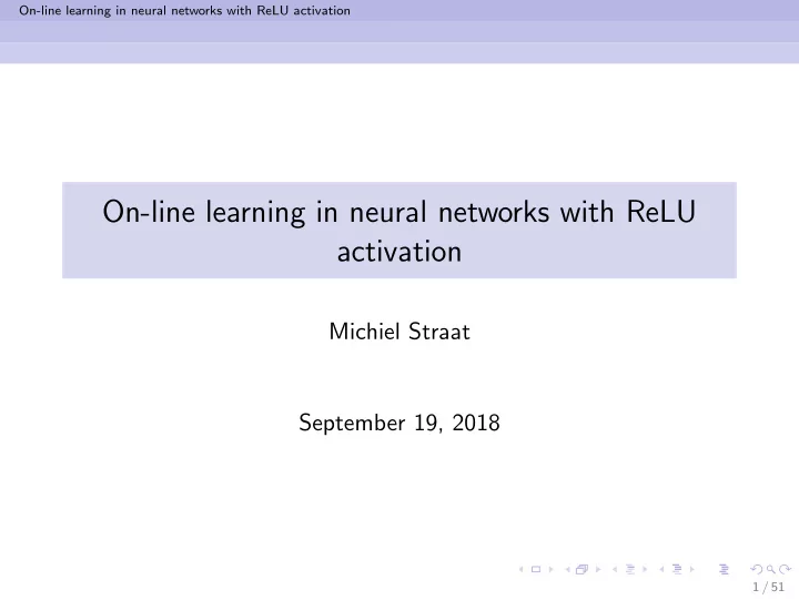
On-line learning in neural networks with ReLU activation On-line learning in neural networks with ReLU activation Michiel Straat September 19, 2018 1 / 51

On-line learning in neural networks with ReLU activation Overview 1 Statistical physics of learning 2 ReLU perceptron learning dynamics 3 ReLU Soft Committee Machine learning dynamics 4 Future research 2 / 51

On-line learning in neural networks with ReLU activation Statistical physics of learning Statistical Mechanics Aims to deduce macroscopic properties from microscopic dynamic properties in systems consisting of e.g. N ≈ 10 23 particles. Due to Central Limit Theorems (CLT), fluctuations in the √ macroscopics become negligible → σ decreases as O (1 / N ) . 3 / 51

On-line learning in neural networks with ReLU activation Statistical physics of learning Example system: Ideal paramagnet ↑↑↓↑↓↑ · · · ↓ Consider N spins, each spin i has a value S i : � � 1 , if ↑ S i = . − 1 , if ↓ Magnetization: N M = 1 � S i ∈ [ − 1 , 1] N i =1 Assume components are i.i.d with P ( S i = 1) = P ( S i = − 1) = 1 2 , � S i � = 0 and σ = 1 . √ CLT: For large N , approximately M ∼ N (0 , 1 / N ) ⇒ M is a deterministic value for N → ∞ (Thermodynamic limit) 4 / 51

On-line learning in neural networks with ReLU activation Statistical physics of learning P ( M ) 40 30 σ = 1 / √ 100 σ = 1 / √ 1000 20 σ = 1 / √ 10000 10 M - 0.3 - 0.2 - 0.1 0.0 0.1 0.2 0.3 5 / 51

On-line learning in neural networks with ReLU activation Statistical physics of learning Statistical Physics of online Learning Online-learning: Uncorrelated examples { ξ µ , τ µ } arrive one at the time. Previously, online learning in Erf neural networks was characterized using methods of Statistical Mechanics. Dynamics of order parameters were formulated, first as difference equations, and in the thermodynamic limit as differential equations. Here, the same method is used to characterize online learning in ReLU neural networks. 6 / 51

On-line learning in neural networks with ReLU activation ReLU perceptron learning dynamics Student-teacher framework The target output τ ( ξ ) is defined by the teacher network. Student tries to learn the rule. g ( · ) is activation function . Input Input layer layer B 1 J 1 ξ 1 ξ 1 τ = g ( B · ξ ) σ = g ( J · ξ ) J 2 B 2 ξ 2 ξ 2 . . . . . . B N J N ξ N ξ N Figure: Teacher with weights Figure: Student with weights B ∈ R N J ∈ R N 7 / 51

On-line learning in neural networks with ReLU activation ReLU perceptron learning dynamics Generalization error Teacher Student Input activation: y µ = B · ξ µ Input activation: x µ = J · ξ µ Output: τ µ = g ( y µ ) Output: σ µ = g ( x µ ) Error on particular example ξ µ 2 ( τ µ − σ µ ) 2 ǫ ( J , ξ µ ) = 1 Generalization error ǫ g ( J ) = � ǫ ( J , ξ ) � ξ where � ... � denotes the average over the input distribution. Assume uncorrelated random components ξ i ∈ N (0 , 1) . 8 / 51

On-line learning in neural networks with ReLU activation ReLU perceptron learning dynamics Gradient descent update rule Upon presentation of an example ξ µ , weight vector J µ is adapted: J µ +1 = J µ − η N ∇ J ǫ ( J µ , ξ µ ) = J µ + η ξ µ = J µ + η N [ g ( y µ ) − g ( x µ )] g ′ ( x µ ) N δ µ ξ µ � �� � δ µ η N is the learning rate scaled by the network size N . Actual form of gradient dependent on choice of g ( · ) 9 / 51

On-line learning in neural networks with ReLU activation ReLU perceptron learning dynamics Order parameters for large dimension N x = J · ξ , y = B · ξ In the limit N → ∞ , the inputs x and y become correlated Gaussian variables according to the Central Limit Theorem, with: � y � = � x � = 0 i = || J || 2 = Q � x 2 � = � N � N j =1 J i J j � ξ i ξ j � = � N i =1 J 2 i =1 � y 2 � = � N � N m =1 B n B m � ξ i ξ j � = � N n = || B || 2 = T = 1 n =1 B 2 n =1 � xy � = � N � N n =1 J i B n � ξ i ξ n � = � N j =1 J j B j = J · B = R i =1 R and Q are the order parameters of the system. 10 / 51

On-line learning in neural networks with ReLU activation ReLU perceptron learning dynamics Updates of the order parameters R µ +1 = J µ +1 · B = ( J µ + η N δ µ ξ µ ) · B � �� � J µ +1 Which leads to the recurrence: R µ +1 = R µ + η N δ µ y µ Updates of order parameters upon presentation of example ξ µ R µ +1 = R µ + η Q µ +1 = Q µ + 2 η N δ µ x µ + η 2 N δ µ y µ , N ( δ µ ) 2 In the limit N → ∞ : The scaled time variable α = µ/N becomes continuous. The order parameters become self-averaging. 11 / 51

On-line learning in neural networks with ReLU activation ReLU perceptron learning dynamics Figure: For fixed α = 20 , the standard deviation of the order parameters R and Q out of 100 runs for increasing system size N . 12 / 51

On-line learning in neural networks with ReLU activation ReLU perceptron learning dynamics N → ∞ (Thermodynamic limit) This results in a system of deterministic differential equations for the evolution of the order parameters: dR dα = η � δy � dQ dα = 2 η � δx � + η 2 � δ 2 � with δ = [ g ( y ) − g ( x )] g ′ ( x ) 13 / 51

On-line learning in neural networks with ReLU activation ReLU perceptron learning dynamics Choice of activation function (b) ReLU activation (a) Erf activation Figure: Examples of perceptrons with different activation for the same weight vector: J 1 = 2 . 5 and J 2 = − 1 . 2 . 14 / 51

On-line learning in neural networks with ReLU activation ReLU perceptron learning dynamics ReLU ReLU activation function Derivative of ReLU x θ ( x ) θ ( x ) 5 1.0 4 0.8 3 0.6 2 0.4 1 0.2 x x - 4 - 2 2 4 - 4 - 2 2 4 (a) g ( x ) = xθ ( x ) (b) g ′ ( x ) = θ ( x ) Figure: The ReLU activation function and its derivative. 15 / 51

On-line learning in neural networks with ReLU activation ReLU perceptron learning dynamics ReLU Perceptron learning dynamics dR dα = η � δy � = η ( � g ′ ( x ) g ( y ) y � − � g ′ ( x ) g ( x ) y � ) = η ( � y 2 θ ( x ) θ ( y ) � − � xyθ ( x ) � ) dQ dα = 2 η � δx � + η 2 � δ 2 � = 2 η ( � g ′ ( x ) g ( y ) x � − � g ′ ( x ) g ( x ) x � ) + η 2 � δ 2 � = 2 η ( � xyθ ( x ) θ ( y ) � − � x 2 θ ( x ) � ) + η 2 � δ 2 � The 2D integrals are taken over the joint Gaussian P ( x, y ) with covariance matrix: � � x 2 � � � Q � � xy � R Σ = = � y 2 � � xy � R 1 16 / 51

On-line learning in neural networks with ReLU activation ReLU perceptron learning dynamics ReLU Perceptron learning dynamics All averages can be expressed analytically in terms of the order parameters. The following system is obtained: � + R √ � T sin − 1 � � R T Q − R 2 √ T Q ∂R T 4 − R ∂α = η 2 + 2 π 2 π Q � √ � sin − 1 � � R R T Q − R 2 √ T Q ∂Q R ∂α = η 2 − Q + + + π π � � √ � sin − 1 � � � R QT − R 2 √ T Q 2 + Q η 2 T R − R Q − 2 + ( T − 2 R ) 4 + 2 π 2 π 2 Integrating the above ODE’s numerically yields the evolution of R ( α ) and Q ( α ) . 17 / 51

On-line learning in neural networks with ReLU activation ReLU perceptron learning dynamics Generalization error ǫ g ( J ) = � ǫ ( J , ξ ) � ξ = 1 2 [ � g ( y ) 2 � − 2 � g ( y ) g ( x ) � + � g ( x ) 2 � ] For ReLU activation, this yields: ǫ g ( J ) = 1 2 [ � y 2 θ ( y ) � − 2 � xyθ ( x ) θ ( y ) � + � x 2 θ ( x ) � ] Performing the averages yields an analytic expression in terms of order parameters R and Q : √ R sin − 1 � � R Q − R 2 √ Q ǫ g ( α ) = 1 + R 4 ) + Q 4 − ( + 2 π 2 π 4 Solving the ODE’s for R ( α ) and Q ( α ) yields evolution of ǫ g ( α ) . 18 / 51

On-line learning in neural networks with ReLU activation ReLU perceptron learning dynamics ReLU perceptron: Results order parameters Evolution R and Q ( ReLU ) Overlap 1.0 ▲ ▲ ▲ ▲ ▲ ▲ ▲ ▲ ▲ ▲ ▲ ▲ ▲ ▲ ▲ ▲ ▲ ▲ ▲ ▲ ▲ ▲ ▲ ▲ ▲ ▲ ▲ ▲ ▲ ▲ ▲ 0.8 ▲ ▲ 0.6 ▲ ▲ R 0.4 ▲ Q ▲ ▲ ▲ 0.2 ▲ α 50 100 150 Figure: solid lines : Theoretical results with R (0) = 0 , Q (0) = 0 . 25 and η = 0 . 1 . Red triangles : Simulation with N = 1000 . 19 / 51

On-line learning in neural networks with ReLU activation ReLU perceptron learning dynamics Generalization error result Generalization error ϵ g ( α ) 0.25 ▲ 0.20 ▲ 0.15 0.10 ▲ 0.05 ▲ ▲ ▲ ▲ ▲ ▲ 0.00 ▲ ▲ ▲ ▲ ▲ ▲ ▲ ▲ ▲ ▲ ▲ α 50 100 150 20 / 51

On-line learning in neural networks with ReLU activation ReLU perceptron learning dynamics Stability perfect solution R = Q = 1 dα = 0 and dQ At R = Q = 1 , dR dα = 0 → fixed point. We consider the linear system � � � R − 1 � − η 0 2 z = F z = ˙ around the fixed 1 − ( η − 1) η 2 ( η − 2) η Q − 1 point. Eigenvalues λ 1 ( η ) = − η 2 and λ 2 ( η ) = 1 2 ( η − 2) η determine stability of the fp. 21 / 51