On a class of dependent Sparre Andersen risk models with - PowerPoint PPT Presentation
Model and Notation The fixed point equation Two applications On a class of dependent Sparre Andersen risk models with application. F.Avram, A.Badescu, M.Pistorius and L.Rabehasaina Laboratory of Mathematics, Besan con, University of
Model and Notation The fixed point equation Two applications On a class of dependent Sparre Andersen risk models with application. F.Avram, A.Badescu, M.Pistorius and L.Rabehasaina Laboratory of Mathematics, Besan¸ con, University of Franche Comt´ e, France. MAM Conference, Budapest, 28th-30th June 2016 1 / 16
Model and Notation The fixed point equation Two applications Content Model and Notation The fixed point equation Two applications 2 / 16
Model and Notation The fixed point equation Two applications Content Model and Notation The fixed point equation Two applications 3 / 16
Model and Notation The fixed point equation Two applications Risk process { X ( t ) , t ≥ 0 } N ( t ) � X ( t ) = u + ct − J k , t ≥ 0 . i =1 N ( t ) = max { n ∈ N : � n k =1 T k ≤ t } number of claims up to time t , T k interclaim, J k claim size, u ≥ 0 initial capital, c > 0 premium rate, c E [ T 1 ] > E [ J 1 ], { ( T k , J k ) , k ∈ N } i.i.d. with dependence structure, defined by P ( T k ∈ d t , J k ∈ d x ) = α ( d t ) e Rx r d x t , x ∈ R + , where α ( d t ) ∈ R 1 × m , is a 1 × m distribution vector, R ∈ R m × m sub-generator matrix, r = ( − R )1. 4 / 16
Model and Notation The fixed point equation Two applications Ruin probability We let τ := { t ≥ 0 , X ( t ) < 0 } the ruin time and its Laplace Transform ˆ e − q τ � � ψ ( q , u ) := E u , q ≥ 0 , u ≥ 0 . → Goal : Compute ˆ − ψ ( q , u ) with efficient algorithm, with LT � ∞ e − qt α ( d t ) ∈ R 1 × m , q ∈ R + , available. α ( − q ) := ˆ 0 Notation : If Q ∈ R m × m negative-definite, we extend definition of LT : � ∞ α ( d t ) e Qt ∈ R 1 × m . α ( Q ) := ˆ 0 α ( − qI ) available for all q ∈ R + , but ˆ ˆ α ( Q ) not explicitly computable in practice for general Q ! 5 / 16
Model and Notation The fixed point equation Two applications Content Model and Notation The fixed point equation Two applications 6 / 16
Model and Notation The fixed point equation Two applications Fixed point equation Theorem Laplace transform ˆ ψ ( q , u ) verifies ˆ ρ ( q ) e [ R + r ˆ ρ ( q )] u 1 , ψ ( q , u ) = ˆ u ≥ 0 , q ≥ 0 , (1) where ˆ ρ ( q ) is a 1 × m sub-probability vector satisfying the fixed point equation ρ ( q ) = ˆ ˆ α ( cR + c r ˆ ρ ( q ) − qI ) , q > 0 . (2) If q = 0 there exists a 1 × m sub-probability vector ˆ ρ (0) verifying (2) such that expression (1) holds for ˆ ψ (0 , u ) . 7 / 16
Model and Notation The fixed point equation Two applications Example and issues Main issue is solving (2), i.e. ρ ( q ) = ˆ ˆ α ( cR + c r ˆ ρ ( q ) − qI ) , ρ ( q ) ∈ R 1 × m subprobability vector. E.g. with unkwown ˆ α ( d t ) ∈ R scalar, J k exponentially distributed : Malinovskii (1998), ˆ ρ ( q ) scalar, α ( d t ) ∈ R scalar, J k ∼ PH ( r , R ) : Asmussen and Albrecher (2010), ˆ ρ ( q ) scalar. Issues here : (2) does not necessarily have a unique solution, 1 α ( d t ) vector, 2 need to be able to compute ˆ α ( M ) where M is a matrix : no 3 explicit form . 8 / 16
Model and Notation The fixed point equation Two applications Algorithm for fixed point equation ρ N ( q ), N ∈ N , solution to Idea : Approximating ˆ ρ ( q ) by ˆ ρ N ( q ) = ˆ α N ( cR + c r ˆ ρ N ( q ) − qI ) , ˆ N M k ( δ )( Q + δ I ) k α N ( Q ) := � where ˆ , δ > 0 large enough, and k ! k =0 � ∞ t k e − δ t α ( d t ) ∈ R 1 × m . M k ( δ ) := 0 9 / 16
Model and Notation The fixed point equation Two applications Algorithm for fixed point equation Advantages : α N ( Q ) computable if the M k ( δ ) ’s, k ∈ N , are computable , − → ˆ − → Convergence : Theorem ρ N ( q ) − One has ˆ → ˆ ρ ( q ) as N → ∞ for all q ≥ 0 . Besides, for q large enough : � N � | M k ( δ ) | m � � ρ N ( q ) � δ k � ˆ ρ ( q ) − ˆ m ≤ C α (0) . 1 − ˆ � � k ! � k =0 with explicit C, and ˆ α (0) explicit. 10 / 16
Model and Notation The fixed point equation Two applications Content Model and Notation The fixed point equation Two applications 11 / 16
Model and Notation The fixed point equation Two applications Bailout problem U 1 ( t ) u 1 Replenishment at level 0 t ζ (1) ζ (1) 1 2 U 0 ( t ) k 1 ζ (1) (prop.cost) 1 u 0 K (1) (fixed cost) 1 k 1 ζ (1) 2 K (1) 2 t Ruin time τ of CB Figure : Sample path with proportional and fixed cost. 12 / 16
Model and Notation The fixed point equation Two applications Bailout problem Goal : Determine LT of ruin time τ of { U 0 ( t ) , t ≥ 0 } ( Central Branch ) starting from u 0 ≥ 0, when claims and interclaims for { U 1 ( t ) , t ≥ 0 } ( subsidiary ) are PH distributed. Step 1 : Identify dependence structure α ( d t ) and matrix R : α ( d t ) ∼ ruin time distribution of τ 1 jointly to phase at ruin , R ∼ same as claims of U 1 ( t ) + independent PH ( k , K ) , − → ˆ α ( − q ), q ∈ R + , available. Step 2 : Compute the M k ( δ )’s, k ∈ N : Ren and Stanford (2012). Step 3 : Run the algorithm. 13 / 16
Model and Notation The fixed point equation Two applications Queues and flushes (in progress) U 1 ( t ) Flush U 0 ( t ) Server Figure : Flush from queue 1 to 0. 14 / 16
Model and Notation The fixed point equation Two applications Queues and flushes Fluid queues { U 0 ( t ) , t ≥ 0 } and { U 1 ( t ) , t ≥ 0 } fluid queues, fed at constant rate c 0 and c 1 . U 1 ( t ) served with priority over U 0 ( t ), instantaneously, according to PH services, Content of U 1 ( t ) is occasionally flushed into U 0 ( t ) at time according to a Poisson process. Goal : Determine LT of ruin time τ of U 0 ( t ) = busy period of U 0 ( t ). Steps : Identify dependence structure α ( d t ) and matrix R , and compute the M k ( δ )’s, k ∈ N . 15 / 16
Model and Notation The fixed point equation Two applications Thank you ! 16 / 16
Recommend
More recommend
Explore More Topics
Stay informed with curated content and fresh updates.


![On the absolute ruin problem in a Sparre Andersen risk model with constant interest [ 1 ] Radu](https://c.sambuz.com/391878/on-the-absolute-ruin-problem-in-a-sparre-andersen-risk-s.webp)
