Numerical integration Recall that Lagrange interpolation of f by n - PowerPoint PPT Presentation

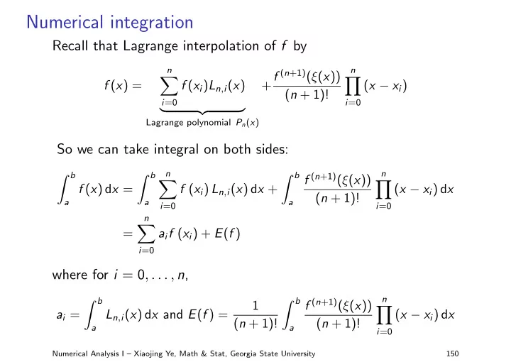
Numerical integration Recall that Lagrange interpolation of f by n n + f ( n +1) ( ξ ( x )) � � f ( x ) = f ( x i ) L n , i ( x ) ( x − x i ) ( n + 1)! i =0 i =0 � �� � Lagrange polynomial P n ( x ) So we can take integral on both sides: � b � b � b n n f ( n +1) ( ξ ( x )) � � f ( x ) d x = f ( x i ) L n , i ( x ) d x + ( x − x i ) d x ( n + 1)! a a a i =0 i =0 n � = a i f ( x i ) + E ( f ) i =0 where for i = 0 , . . . , n , � b � b n f ( n +1) ( ξ ( x )) 1 � a i = L n , i ( x ) d x and E ( f ) = ( x − x i ) d x ( n + 1)! ( n + 1)! a a i =0 Numerical Analysis I – Xiaojing Ye, Math & Stat, Georgia State University 150

Trapezoidal rule Suppose we know f at x 0 = a and x 1 = b , then P 1 ( x ) = ( x − x 1 ) ( x 0 − x 1 ) f ( x 0 ) + ( x − x 0 ) ( x 1 − x 0 ) f ( x 1 ) Then taking integral of f yields � ( x − x 1 ) � b � x 1 � ( x 0 − x 1 ) f ( x 0 ) + ( x − x 0 ) f ( x ) d x = ( x 1 − x 0 ) f ( x 1 ) d x a x 0 � x 1 + 1 f ′′ ( ξ ( x )) ( x − x 0 ) ( x − x 1 ) d x 2 x 0 Numerical Analysis I – Xiaojing Ye, Math & Stat, Georgia State University 151

Trapezoidal rule Integral of the first term on the right is straightforward. Note that the second term on the right is � x 1 f ′′ ( ξ ( x )) ( x − x 0 ) ( x − x 1 ) d x x 0 � x 1 = f ′′ ( ξ ) ( x − x 0 ) ( x − x 1 ) d x x 0 � � x 1 x 3 3 − ( x 1 + x 0 ) x 2 + x 0 x 1 x = f ′′ ( ξ ) 2 x 0 = − h 3 6 f ′′ ( ξ ) where ξ ∈ ( x 0 , x 1 ) by MVT for integrals and Numerical Analysis I – Xiaojing Ye, Math & Stat, Georgia State University 152

Trapezoidal rule Therefore, we obtain � � x 1 � b 2 ( x 0 − x 1 ) f ( x 0 ) + ( x − x 0 ) 2 ( x − x 1 ) 2 − h 3 12 f ′′ ( ξ ) f ( x ) dx = 2 ( x 1 − x 0 ) f ( x 1 ) a x 0 − h 3 = ( x 1 − x 0 ) � � 12 f ′′ ( ξ ) f ( x 0 ) + f ( x 1 ) 2 Trapezoidal rule: � b − h 3 f ( x ) d x = h � � 12 f ′′ ( ξ ) f ( x 0 ) + f ( x 1 ) 2 a Numerical Analysis I – Xiaojing Ye, Math & Stat, Georgia State University 153

Trapezoidal rule Illustration of Trapezoidal rule: y y � f ( x ) y � P 1 ( x ) a � x 0 x x 1 � b Numerical Analysis I – Xiaojing Ye, Math & Stat, Georgia State University 154

Simpson’s rule If we have values of f at x 0 = a , x 1 = a + b 2 , and x 2 = b . Then � ( x − x 1 ) ( x − x 2 ) � b � x 2 ( x 0 − x 1 ) ( x 0 − x 2 ) f ( x 0 ) + ( x − x 0 ) ( x − x 2 ) f ( x ) d x = ( x 1 − x 0 ) ( x 1 − x 2 ) f ( x 1 ) a x 0 + ( x − x 0 ) ( x − x 1 ) ( x 2 − x 0 ) ( x 2 − x 1 ) f ( x 2 )] d x � x 2 ( x − x 0 ) ( x − x 1 ) ( x − x 2 ) f (3) ( ξ ( x )) d x + 6 x 0 Numerical Analysis I – Xiaojing Ye, Math & Stat, Georgia State University 155

Simpson’s rule With similar idea, we can derive the Simpson’s rule : � x 2 − h 5 f ( x ) dx = h � � 90 f (4) ( ξ ) f ( x 0 ) + 4 f ( x 1 ) + f ( x 2 ) 3 x 0 y y � f ( x ) y � P 2 ( x ) x a � x 0 x 1 x 2 � b Numerical Analysis I – Xiaojing Ye, Math & Stat, Georgia State University 156

Example Example (Trapezoidal and Simpson’s rules for integration) � 2 Compare Trapezoidal and Simpson’s rules on 0 f ( x ) d x where f is (a) x 2 (b) x 4 (c) ( x + 1) − 1 √ (f) e x 1 + x 2 (d) (e) sin x Solution. Apply the the formulas respectively to get: (a) (b) (c) (d) (e) (f) Problem √ x 2 x 4 ( x + 1) − 1 e x 1 + x 2 f ( x ) sin x Exact value 2.667 6.400 1.099 2.958 1.416 6.389 4.000 16.000 1.333 3.326 0.909 8.389 Trapezoidal 2.667 6.667 1.111 2.964 1.425 6.421 Simpson’s Numerical Analysis I – Xiaojing Ye, Math & Stat, Georgia State University 157

Newton-Cotes formula We can follow the same idea to get higher-order approximations, called the Netwon-Cotes formulas. For n = 3 where ξ ∈ ( x 0 , x 3 ): � x 3 − 3 h 5 f ( x ) d x = 3 h � � 80 f (4) ( ξ ) f ( x 0 ) + 3 f ( x 1 ) + 3 f ( x 2 ) + f ( x 3 ) 8 x 0 For n = 4 where ξ ∈ ( x 0 , x 4 ): � x 4 f ( x ) d x =2 h � � 7 f ( x 0 ) + 32 f ( x 1 ) + 12 f ( x 2 ) + 32 f ( x 3 ) + 7 f ( x 4 ) 45 x 0 − 8 h 7 945 f (6) ( ξ ) Numerical Analysis I – Xiaojing Ye, Math & Stat, Georgia State University 158

Composite numerical integration Problem with Newton-Cotes rule for high degree is oscillations. y y = P n ( x) y = f ( x) x a � x 0 x 1 x 2 x n � 1 x n � b Instead, we can approximate the integral “piecewisely”. Numerical Analysis I – Xiaojing Ye, Math & Stat, Georgia State University 159

Composite midpoint rule Let x − 1 = a , x 0 , x 1 , . . . , x n , x n +1 = b be a uniform partition of [ a , b ] with h = b − a n +2 . Then we obtain the composite midpoint rule : � b n / 2 + b − a � � � h 2 f ′′ ( µ ) f ( x ) d x = 2 h f x 2 j 6 a j =0 y y � f ( x ) x 2 j x 2 j � 1 b � x n � 1 x a � x � 1 x 0 x 1 x 2 j � 1 x n � 1 x n Numerical Analysis I – Xiaojing Ye, Math & Stat, Georgia State University 160

Composite trapezoidal rule Let x 0 = a , x 1 , . . . , x n = b be a uniform partition of [ a , b ] with h = b − a n . Then we obtain the composite Trapezoidal rule :   � b n − 1  − b − a f ( x ) d x = h � � � 12 h 2 f ′′ ( µ )  f ( a ) + 2 + f ( b ) f x j 2 a j =1 y y � f ( x ) x a � x 0 x 1 x j � 1 x j x n � 1 b � x n Numerical Analysis I – Xiaojing Ye, Math & Stat, Georgia State University 161

Composite Simpson’s rule Let x 0 , x 1 , . . . , x n ( n even) be a uniform partition of [ a , b ]. Then apply Simpson’s rule on [ x 0 , x 2 ] , [ x 2 , x 4 ] , . . . , a total of n such intervals. Then we obtain the composite Simpson’s rule :   � b ( n / 2) − 1 n / 2 f ( x ) dx = h  − b − a � � 180 h 4 f (4) ( µ )  f ( a ) + 2 f ( x 2 j ) + 4 f ( x 2 j − 1 ) + f ( b ) 3 a j =1 j =1 y y � f ( x ) x a � x 0 x 2 x 2 j � 2 x 2 j � 1 x 2 j b � x n Numerical Analysis I – Xiaojing Ye, Math & Stat, Georgia State University 162

Gauss quadrature Previously we chose points (nodes) with fixed gaps. What if we are allowed to to choose points x 0 , . . . , x n and evaluate f there? y y y y � f ( x ) y � f ( x ) y � f ( x ) x x x a � x 1 x 2 � b a � x 1 x 2 � b a � x 1 x 2 � b y y y y � f ( x ) y � f ( x ) y � f ( x ) x x x a x 1 x 2 b a x 1 x 2 b a x 1 x 2 b Numerical Analysis I – Xiaojing Ye, Math & Stat, Georgia State University 163

Gauss quadrature Gauss quadrature tries to determine x 1 , . . . , x n and c 1 , . . . , c n s.t. � b n � f ( x ) d x ≈ c i f ( x i ) a i =1 Conceptually, since we have 2 n parameters, i.e., c i , x i for i = 1 , . . . , n , we expect to get “=” if f ( x ) is a polynomial of degree ≤ 2 n − 1. Numerical Analysis I – Xiaojing Ye, Math & Stat, Georgia State University 164

Gauss quadrature Let’s first try the case with interval [ − 1 , 1] and two points x 1 , x 2 ∈ [ − 1 , 1]. Then we need to find x 1 , x 2 , c 1 , c 2 such that � 1 f ( x ) dx ≈ c 1 f ( x 1 ) + c 2 f ( x 2 ) − 1 and “=” holds for all polynomials of degree ≤ 3. Numerical Analysis I – Xiaojing Ye, Math & Stat, Georgia State University 165

Gauss quadrature We first note � � � � � � a 0 + a 1 x + a 2 x 2 + a 3 x 3 � x 2 d x + a 3 x 3 d x d x = a 0 1 d x + a 1 x d x + a 2 � 1 Then we need x 1 , x 2 , c 1 , c 2 s.t. − 1 f ( x ) d x = c 1 f ( x 1 ) + c 2 f ( x 2 ) for f ( x ) = 1 , x , x 2 , and x 3 : � 1 c 1 · 1 + c 2 · 1 = 1 d x = 2 , − 1 � 1 c 1 · x 1 + c 2 · x 2 = x d x = 0 − 1 � 1 x 2 d x = 2 c 1 · x 2 1 + c 2 · x 2 2 = 3 , − 1 � 1 x 3 d x = 0 c 1 · x 3 1 + c 2 · x 3 2 = − 1 Numerical Analysis I – Xiaojing Ye, Math & Stat, Georgia State University 166

Gauss quadrature Solve the system of four equations to obtain x 1 , x 2 , c 1 , c 2 : √ √ 3 3 c 1 = 1 , c 2 = 1 , x 1 = − and x 2 = 3 , 3 So the approximation is √ � √ � � � � 1 − 3 3 f ( x ) d x ≈ f + f 3 3 − 1 which is exact for all polynomials of degree ≤ 3. This point and weight selection is called Gauss quadrature . Numerical Analysis I – Xiaojing Ye, Math & Stat, Georgia State University 167

Legendre polynomials To obtain Gauss quadrature for larger n , we need Legendre polynomials { P n : n = 0 , 1 , . . . } : 1. All P n are monic (leading coefficient =1) 2. � 1 P ( x ) P n ( x ) d x = 0 − 1 for all polynomial P of degree less than n . Numerical Analysis I – Xiaojing Ye, Math & Stat, Georgia State University 168

Legendre polynomials The first five Legendre polynomials: P 0 ( x ) = 1 P 1 ( x ) = x P 2 ( x ) = x 2 − 1 3 P 3 ( x ) = x 3 − 3 5 x P 4 ( x ) = x 4 − 6 7 x 2 + 3 35 Numerical Analysis I – Xiaojing Ye, Math & Stat, Georgia State University 169

Gauss quadrature and Legendre polynomial Theorem (Obtain Gauss quadrature by Legendre poly.) Suppose x 1 , . . . , x n are the roots of the nth Legendre polynomial P n ( x ) , and define � 1 n x − x j � c i = d x x i − x j − 1 j =1 j � = i If P ( x ) is any polynomial of degree less than 2 n, then � 1 n � P ( x ) dx = c i P ( x i ) − 1 i =1 Numerical Analysis I – Xiaojing Ye, Math & Stat, Georgia State University 170