MATH 3341: Introduction to Scientific Computing Lab Libao Jin - PowerPoint PPT Presentation
Lab 12: Romberg Integration MATH 3341: Introduction to Scientific Computing Lab Libao Jin University of Wyoming April 29, 2020 L. Jin MATH 3341 Lab 12: Romberg Integration Romberg Integration Lab 12: Romberg Integration L. Jin MATH 3341
Lab 12: Romberg Integration MATH 3341: Introduction to Scientific Computing Lab Libao Jin University of Wyoming April 29, 2020 L. Jin MATH 3341
Lab 12: Romberg Integration Romberg Integration Lab 12: Romberg Integration L. Jin MATH 3341
Lab 12: Romberg Integration Romberg Integration Romberg Integration L. Jin MATH 3341
Lab 12: Romberg Integration Romberg Integration Composite Trapezoidal rule for approximating the integral of a function f ( x ) on an interval [ a, b ] using m subintervals is � b m − 1 f ( x ) dx = h − b − a � 12 h 2 f ′′ ( ξ ) , f ( a ) + f ( b ) + 2 f ( x j ) 2 a j =1 where a ≤ ξ ≤ b and h = ( b − a ) /m and x j = a + jh for each j = 0 , 1 , . . . , m . L. Jin MATH 3341
Lab 12: Romberg Integration Romberg Integration Finding approximation for m 1 = 1 , m 2 = 2 , m 3 = 4 , . . . , m n = 2 n − 1 for n ∈ N . The corresponding step size h k for each m k is then given by h k = ( b − a ) /m k = ( b − a ) / 2 k − 1 . The trapezoidal rule then becomes � b 2 k − 1 − 1 f ( x ) dx = h k − b − a � 12 h 2 f ′′ ( ξ k ) , f ( a ) + f ( b ) + 2 f ( a + jh k ) 2 a j =1 where ξ k ∈ [ a, b ] . L. Jin MATH 3341
Lab 12: Romberg Integration Romberg Integration Here we’ll use the notation R k, 1 to denote the portion used for the trapezoidal approximation. In other words, R 1 , 1 = h 1 2 [ f ( a ) + f ( b )] = b − a [ f ( a ) + f ( b )] , 2 R 2 , 1 = h 2 2 [ f ( a ) + f ( b ) + 2 f ( a + h 2 )] = 1 b − a a + b − a � � �� f ( a ) + f ( b ) + 2 f 2 2 2 = 1 2[ R 1 , 1 + h 1 f ( a + h 2 )] , R 3 , 1 = 1 2 { R 2 , 1 + h 2 [ f ( a + h 3 ) + f ( a + 3 h 3 )] } . L. Jin MATH 3341
Lab 12: Romberg Integration Romberg Integration This leads to the Trapezoidal rule in the general form 2 k − 2 R k, 1 = 1 � R k − 1 , 1 + h k − 1 f ( a + (2 j − 1) h k ) for k = 2 , 3 , . . . , n. 2 j =1 This method converges very slowly on its own. A technique called Richardson’s Extrapolation is applied to speed convergence. Essentially, this performs a method of averaging previously calculated entries to obtain the next entry in the table. This is given in general form R k,j = R k,j − 1 + R k,j − 1 − R k − 1 ,j − 1 . 4 j − 1 − 1 L. Jin MATH 3341
Lab 12: Romberg Integration Romberg Integration This method will give us the following entries of R in a tabular format. The number of rows is determined by the value that we desire. R 1 , 1 R 2 , 1 R 2 , 2 R 3 , 1 R 3 , 2 R 3 , 3 R 4 , 1 R 4 , 2 R 4 , 3 R 4 , 4 . . . . ... . . . . . . . . R n, 1 R n, 2 R n, 3 R n, 4 · · · R n,n L. Jin MATH 3341
Lab 12: Romberg Integration Romberg Integration Algorithm Algorithm 1: Romberg Integration Function romberg( f, a, b, n ) : h ← b − a ; R 1 , 1 ← [ f ( a ) + f ( b )] · h/ 2 ; for k ← 2 to n do 2 k − 2 R k, 1 ← 1 � R k − 1 , 1 + h f ( a + (2 j − 1) · h/ 2) ; 2 j =1 for j ← 2 to k do R k,j ← R k,j − 1 + R k,j − 1 − R k − 1 ,j − 1 ; 4 j − 1 − 1 end h ← h/ 2 ; end return [ R 1 , 1 , R 2 , 2 , R 3 , 3 , . . . , R n,n ] ; end L. Jin MATH 3341
Recommend
More recommend
Explore More Topics
Stay informed with curated content and fresh updates.
