Numerical Integration and Monte Carlo Integration Elementary - PowerPoint PPT Presentation

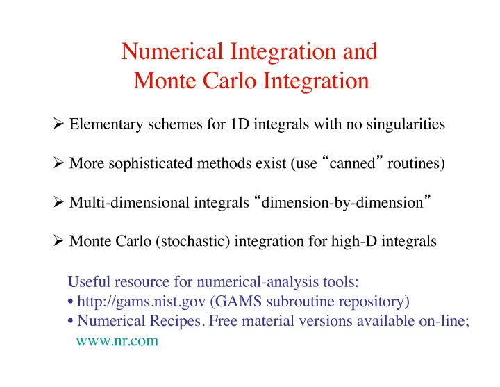
Numerical Integration and Monte Carlo Integration Ø Elementary schemes for 1D integrals with no singularities Ø More sophisticated methods exist (use “ canned ” routines) Ø Multi-dimensional integrals “ dimension-by-dimension ” Ø Monte Carlo (stochastic) integration for high-D integrals Useful resource for numerical-analysis tools: • http://gams.nist.gov (GAMS subroutine repository) • Numerical Recipes. Free material versions available on-line; www.nr.com

Numerical integration; 1D methods • Assuming that the integrand has no singularities • Discretize: • Fit N-th order polynomial to N+1 points; integrate pieces • Error typically

N=1 Solving this gives: Integrating; This is called the trapezoidal rule

N=2 Solving for a,b,c and integrating --> Simpson ’ s rule

Extended trapezoidal and Simpson ’ s rules Extended open formulas (boundaries excluded):

Integrable singularities Ø The open formulas discussed can be used Ø Error scaling with h will be worse Ø Some singularities can be transformed away Ø Asymptotic divergence can some times be subtracted (analytically solvable, leaving non-singular integral) Ø More sophisticated methods exist for difficult cases Simpson ’ s rule is adequate for many “ proper ” integrals If faster convergence needed -- Romberg integration

Romberg integration Idea: Use trapezoidal rule with different h Ø Error scales as h 2 (+ higher-order terms) Ø Only even powers , i.e., polynomial in h 2 Ø Extrapolate to h=0 using interpolating polynomial Simplest case; n=1, use h=h 0 and h=h 0 /2 Extrapolate to zero leading error (solving for ): Equivalent to Simpson ’ s rule! Trick: Doubling number of points (h k+1 = h k /2) Ø old points can be used; factor-2 time-savings

High-order Romberg integration Need polynomial interpolating between n approximants; Lagrange ’ s formula for n points (x i ,y i ): Error is polynomial in x=h 2 , h=h 0 /2 k ; evaluate polynomial at x=0 Remaining error is Very rapid convergence!

Program implementation of Romberg ’ s method Trapezoidal rule with point-doubling • integrates from x0 to xn; old and new result in trap • start with n+1 points (n segments) subroutine trapezoidal(x0,xn,n,trap,step) integer :: i,n,step real(8) :: h,h2,x0,xn,x0h,trap,func h=(xn-x0)/dble(n*2**step) if (step == 0) then trap=0.5d0*(func(x0)+func(xn)) do i=1,n-1 trap=trap+func(x0+h*dble(i)) enddo else h2=2.d0*h x0h=x0+h trap=trap/h2 ! trap contains old (n-1) result do i=0,n*2**(step-1)-1 trap=trap+func(x0h+h2*dble(i)) enddo endif trap=trap*h

Extrapolating trapezoidal approximants 0,..,n function polext(n,y) integer :: j,k,n real(8) :: y(0:n),p,polext polext=0.d0 do k=0,n p=1.d0 do j=0,n if (j /= k) p=p/(2.d0**(2*(j-k))-1.d0) enddo polext=polext+p*y(k)*(-1)**n enddo Loop in main program do i=0,steps-1 call trapezoidal(x0,xn,n,t,i) trap(i)=t if (i /= 0) print*,trap(i),polext(i,trap) enddo

Multi-dimensional Integration Can be carried out “ dimension-by-dimension ” using 1D method 2D example with non-rectangular boundaries: Can be written as 1D y-integral of function that is an x-integral Very time-consuming for D > 3. Scaling: M 1 =time for 1D