[PPT] - Numerical Approach on Hydrogen Numerical Approach on Hydrogen PowerPoint Presentation

SLIDE 1

1 1

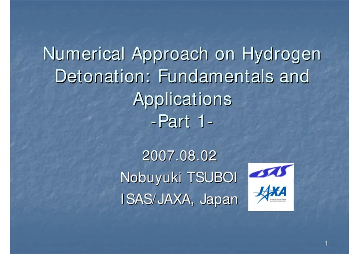
Numerical Approach on Hydrogen Numerical Approach on Hydrogen Detonation: Fundamentals and Detonation: Fundamentals and Applications Applications

Part 1

Part 1-

2007.08.02

2007.08.02 Nobuyuki TSUBOI Nobuyuki TSUBOI ISAS/JAXA, Japan ISAS/JAXA, Japan

SLIDE 2

2 2

1.Motivations

2. Numerical simulation for compressible

high speed flow (1) Scalar equations (2) System equations (3) System equations with chemical reactions 3.Summary

Overview Overview

SLIDE 3

3 3

Motivations Motivations

1.Hydrogen/air mixture: detonable gas 2.Detonation: shock induced combustion

Pressure behind detonation increases

about 10 times ambient pressure 3.Closed environment such as a tunnel causes serious accident.

SLIDE 4

4 4

Numerical Simulations Numerical Simulations

1.Detonation as well as thermal and gas dynamic phenomena of airplane and aerospace plane are elucidated numerically.

2. Main issues

(1) Robust numerical scheme for high pressure and temperature (2) Stiff problem: chemical characteristic time is much faster than the fluid characteristic time (3) Chemical reaction model for high pressure combustion (4) Unsteadiness, turbulence, and three- dimensional problems

SLIDE 5

5 5

Flow Chart of Numerical Simulations Flow Chart of Numerical Simulations

Computational Grid Program Visualization Physical Model？ Flowfield to Simulate？ Mathematical Model？ Discretization？ Submit Job

・・Compressible? Incompressible? Chemical reaction? Turbulence? ・・Euler equations？ Navier-Stokes equations？・・Finite difference？Finite Volume？ Finite element？・・Structure grid？Unstructure grid？ Cartesian grid？・・Supercomputer? Workstation? ・・Workstation? Personal computer? ・・Fortran? C?

SLIDE 6

6 6

Conceptual Conceptual design design

w/o separation w/o separation less turbulence less turbulence Panel Method Panel Method Potential Potential Eq Eq. .

Academic Academic research research Academic Academic research research Academic Academic research, research, Detailed Detailed design design Conceptual Conceptual design design Level Level

Solve all vortices Solve all vortices DNS(Direct DNS(Direct Numerical Numerical Simulation) Simulation) Solve scale Solve scale vortices smaller vortices smaller than grid than grid LES(Large LES(Large Eddy Simulation) Eddy Simulation) Boundary layer, Boundary layer, separation separation RANS(Reynolds RANS(Reynolds averaged averaged Navier Navier-

Stokes

Stokes Eq Eq.) .) Shock Shock Euler Euler Eq Eq. . Target Target Mathematical Model Mathematical Model

Numerical Model Numerical Model

SLIDE 7

7 7

Structured grid ? Unstructured grid ? Cartesian grid ? How to make grids ? ・・Commercial software ? ・・Make by oneself ?

Computational Grids Computational Grids

SLIDE 8

8 8

Flowchart of program is defined after discretization and grid are decided

Start Initialization Boundary condition Define time step Calculate numerical flux Calculate time integration Convergence ? Output data End

No

Read grid, parameter, and set initial condition Output simulation results CFL number Convective flux, viscous term Upwind method, central difference, Higher-order Explicit or implicit time integration

Numerical analysis for fluid: finite different method Numerical analysis for fluid: finite different method

SLIDE 9

9 9

Scalar Equation Scalar Equation

SLIDE 10

10 10

Wave equation ・・ wave propagates with speed, c u x c u2 u1

Finite Difference for Scalar Equation Finite Difference for Scalar Equation

u u c t x ∂ ∂ + = ∂ ∂

SLIDE 11

11 11

( )

) ( 2 2 1

1 1 1 1 1 n j n j n j n j n j

u u x t c u u u

− + + − +

− ⎟ ⎠ ⎞ ⎜ ⎝ ⎛ Δ Δ − + = ) ( 2

1 1 1 n j n j n j n j

u u x t c u u

− + +

− ⎟ ⎠ ⎞ ⎜ ⎝ ⎛ Δ Δ − =

FTCS (Forward in Time and Central Difference in Space)

・・Explicit+central difference:unstable

⎟ ⎠ ⎞ ⎜ ⎝ ⎛ Δ Δ = x t c ν

・・CFL number: parameter to govern numerical stability

First-order upwind method (Upwind difference)

) (

1 1 n j n j n j n j

u u x t c u u

− +

− ⎟ ⎠ ⎞ ⎜ ⎝ ⎛ Δ Δ − =

・・Find direction which wave propagates and use upwind data only

Lax method

More stable than FTCS Large numerical dissipation

Lax-Wendroff method 2nd order in space and time

u u c t x ∂ ∂ + = ∂ ∂

( ) ( )

2 2 1 1 1 1 1

2 2 2

n n n n n n n j j j j j j j

c t c t u u u u u u u x x

+ + − + −

Δ Δ ⎛ ⎞ ⎛ ⎞ = − − + − + ⎜ ⎟ ⎜ ⎟ Δ Δ ⎝ ⎠ ⎝ ⎠

SLIDE 12

12 12

Pseudo-finite volume method ・Conservation form ・・Non-linear equation with discontinuous wave can be calculate and discreted ・・Compressible equations is based on this concept

0, u f f cu t x ∂ ∂ + = = ∂ ∂

1 − j

Flux

j 1 + j

2 1

− j

2 1

+ j

( )

1 1/2 1/2 n n n n j j j j

t u u f f x

+ + −

Δ ⎛ ⎞ = − − ⎜ ⎟ Δ ⎝ ⎠ % %

n j

f

2 / 1

~

+

：Numerical flux

n j

f

2 / 1

~

+ 1/ 2 n j

f − %

SLIDE 13

13 13

( )

1 1/2 1/2 n n n n j j j j

t u u f f x

+ + −

Δ ⎛ ⎞ = − − ⎜ ⎟ Δ ⎝ ⎠ % %

( ) ( )

1/2 1 1

1 2 2

n n n n n j j j j j

c f f f u u

+ + +

= + = + %

For example, FTCS is applied,

( ) ( ) ( )

{ }

( )

1 1 1 1 1 1/2 1/ 2

2 1 2

n n n n j j j j n n n n n j j j j j n n n j j j

c t u u u u x t u cu cu cu cu x t u f f x

+ + − + − + −

Δ ⎛ ⎞ = − − ⎜ ⎟ Δ ⎝ ⎠ Δ ⎛ ⎞ = − + − + ⎜ ⎟ Δ ⎝ ⎠ Δ ⎛ ⎞ = − − ⎜ ⎟ Δ ⎝ ⎠ % %

Therefore

SLIDE 14

14 14

There exist many numerical schemes, however, these schemes are designed how to estimate numerical flux

n j

f

2 / 1

~

+

FTCS

˜ f

j+1 / 2 n

= 1 2 ( fj+1

n + fj n) = c

2 (uj+1

n

+ uj

n)

Lax

) ( 2 1 ) ( 2 ~

1 1 2 / 1 n j n j n j n j n j

u u t x u u c f − ⎟ ⎠ ⎞ ⎜ ⎝ ⎛ Δ Δ − + =

+ + +

1st order upwind difference ˜ f

j +1 / 2 n

= c 2 (uj +1

n

+ uj

n) − c

2 (uj+1

n

− uj

n) = cuj n = fj n

)] )( 1 ( 2 1 [ ) 1 ( 2 ) 1 ( 2 ~

1 1 2 / 1 j j j j j n j

u u u c u c u c f − − + = − + + =

+ + +

ν ν ν

Lax-Wendroff

⎟ ⎠ ⎞ ⎜ ⎝ ⎛ Δ Δ = x t c ν

SLIDE 15

15 15

1st order upwind difference

˜ f

j+1 / 2 n

= c 2 (uj+1

n

+ uj

n) − c

2 (uj+1

n

− uj

n) = cuj n = fj n

⎪ ⎩ ⎪ ⎨ ⎧ ≤ ≤ =

+ +

, , ~

1 2 / 1

c f c f f

n j n j n j

When sign of c is unclear, summarized as follows:

[ ] [ ]

) ( ) ( 2 1 ) ( ) ( 2 1 2 2 ~

1 1 1 1 1 2 / 1 j j j j j j j j j j n j

u u c f f u u c cu cu u c c u c c f − − + = − − + = + + − =

+ + + + + +

SLIDE 16

16 16

1st order upwind difference

˜ f

j +1 / 2 n

= cuj

n

Lax-Wendroff

)] )( 1 ( 2 1 [ ) 1 ( 2 ) 1 ( 2 ~

1 1 2 / 1 j j j j j n j

u u u c u c u c f − − + = − + + =

+ + +

ν ν ν

L-W scheme = 1st order upwind + modified flux

> 2nd order

TVD(Total TVD(Total Variation Variation Dimishing Dimishing) Method ) Method

SLIDE 17

17 17

)] )( 1 ( 2 1 [ ~

1 2 / 1 j j j n j

u u u c f − − + =

+ +

ν

modified flux

L-W scheme generates numerical oscillation. Another scheme added non-linear flux is introduced.

~ [ ( )( )]

/ /

f c u B u u

j n j j j j + + +

= + − −

1 2 1 2 1

1 2 1 ν

flux limiter function

When B select well, monotone scheme, which is almost higher order and becomes 1st order near discontinuity, can be created ・・Modified flux method proposed by Harten

1 ( ) (1 ) 2 c c σ ν ≅ −

SLIDE 18

18 18

u x Monotone imply a property to become 1st order near discontinuity monotone solution non-monotone solution

What is monotone scheme? What is monotone scheme?

SLIDE 19

19 19

TV(u

n) =

uj+1

n

− uj

n j

∑

TV(u

n+1) ≤ TV(u n)

Total variation in space at a time defines as follows: TV stability：Total variation decrease with time (diminishing)・・TVD condition Scheme which is satisfied this condition is called TVD scheme. ：Total variation

TVD(Total TVD(Total Variation Diminishing) Method Variation Diminishing) Method

SLIDE 20

20 20

TVD scheme means to preserve monotone profile For example, 1st order upwind difference is TVD scheme. In order to preserve monotone,

uj

n+1 = uj n + Δt

Δx[cj +1 / 2

−

(uj +1 − uj) + cj −1/ 2

+

(uj − uj −1)] cj +1/ 2

−

> 0, cj −1/ 2

+

> 0, Δt Δx (cj +1/ 2

−

− cj −1/ 2

+

) ≤ 1

monotone TVD scheme CFL condition

TVD(Total TVD(Total Variation Diminishing) Method Variation Diminishing) Method

SLIDE 21

21 21

⎪ ⎩ ⎪ ⎨ ⎧ ≤ = ≤ = =

+ + +

, , ~

1 1 2 / 1

c cu f c cu f f

n j n j n j n j n j

From piecewise constant in cell to piecewise linear in cell ・・cause oscillate solutions!

piecewise constant piecewise linear

j-2 j-1 j j+1 uj-2 uj-1 uj uj+1 j-1 j j+1 j+2 uj-1 uj uj+1 uj+2

1/ 2 L j

u +

1/ 2 R j

u +

Higher order Numerical Flux Higher order Numerical Flux

SLIDE 22

22 22

1st order 2nd order 1st order 2st order

Non-MUSCL+limiter, TVD MUSCL+limiter, TVD

u u

) ( ~ u f ) ( ~ u f

MUSCL:Monotone Upstream-centred Schemes for Conservation Laws

Higher order Numerical Flux Higher order Numerical Flux

j-1 j j+1 j+2 uj-1 uj uj+1 uj+2

1/ 2 L j

u +

1/2 R j

u +

SLIDE 23

23 23

System Equation System Equation

SLIDE 24

24 24

Define flowchart of program after discretization and grid are decided

Start Initialization Boundary condition Define time step Calculate numerical flux Calculate time integration Convergence ? Output data End

No

Read grid, parameter, and set initial condition Output simulation results CFL number Convective flux, viscous term Upwind method, central difference, Higher-order Explicit or implicit time integration

Numerical Analysis for Fluid: Finite Different Method Numerical Analysis for Fluid: Finite Different Method

SLIDE 25

25 25

Solution of system equations Solution of scalar equation

・Non-linear

Previous discussion assumed as linear equation

・Simultaneous equations

Difficult to find the upwind direction

Therefore, ・Linearization is necessary ・Decompose to some wave equations in order to define the upwind direction

SLIDE 26

26 26

Mass conservation Momentum conservation Energy conservation 1-D Compressible Euler Equations

e p h H ρ + = =

Enthalpy per unit mass

p RT ρ =

Equation of State (Ideal Gas)

where

( )

u t x ρ ρ ∂ ∂ + = ∂ ∂

( )

2

u p u t x ρ ρ ∂ + ∂ + = ∂ ∂

( )

e p u e t x ∂ + ∂ + = ∂ ∂

Discretization Discretization of System Equations

f System Equations

SLIDE 27

27 27

where, (ideal gas)

1 1 1 1

v

p E RT C T γ ρ γ = = = − −

Internal energy per unit mass Enthalpy per unit mass

2 2 2 2

1 1 1 2 1 1 1 1 2 1 2 2

p

h e p p H u p p u RT u C T u ρ ρ ρ ρ γ γ γ γ ρ γ ⎛ ⎞ + = = = + + ⎜ ⎟ − ⎝ ⎠ = + = + = + − −

Enthalpy per unit volume

2 2

2 1 1 ) 2 ( u P u E e ρ γ ρ + − = + =

SLIDE 28

28 28

Q E t x ∂ ∂ + = ∂ ∂

Vector form of governing equations:

⎟ ⎟ ⎟ ⎠ ⎞ ⎜ ⎜ ⎜ ⎝ ⎛ + + = ⎟ ⎟ ⎟ ⎠ ⎞ ⎜ ⎜ ⎜ ⎝ ⎛ = u p e u p u E e u Q ) ( ,

2

ρ ρ ρ ρ

⎥ ⎥ ⎥ ⎥ ⎦ ⎤ ⎢ ⎢ ⎢ ⎢ ⎣ ⎡ + + = ⎥ ⎥ ⎥ ⎥ ⎦ ⎤ ⎢ ⎢ ⎢ ⎢ ⎣ ⎡ + + = ⎥ ⎥ ⎥ ⎥ ⎦ ⎤ ⎢ ⎢ ⎢ ⎢ ⎣ ⎡ = v p e v p vu v F u p e uv u p u E e v u Q ) ( , ) ( ,

2 2

ρ ρ ρ ρ ρ ρ ρ ρ ρ

1-D 2-D

Q E F t x y ∂ ∂ ∂ + + = ∂ ∂ ∂

SLIDE 29

29 29

Governing equation is linearlized

⎟ ⎟ ⎟ ⎟ ⎟ ⎟ ⎠ ⎞ ⎜ ⎜ ⎜ ⎜ ⎜ ⎜ ⎝ ⎛ − − − − − − − − = ∂ ∂ = u u h u h u u u Q E A ρ ρ ρ ρ γ ρ

2 2 2

) 1 ( ) 2 1 ( 1 ) 3 ( 2 3 1

Q E t x ∂ ∂ + = ∂ ∂ Q Q A t x ∂ ∂ + = ∂ ∂

SLIDE 30

30 30

Property of 1-D Euler equations Derive eigen value

w w A r r λ =

λ

) 1 ( ) 2 1 ( 1 ) 3 ( 2 3 1

2 2 2

= − − − − − − − − − − − λ ρ ρ ρ ρ λ γ ρ λ u u h u h u u u

) ( ) (

2

= ⎟ ⎟ ⎠ ⎞ ⎜ ⎜ ⎝ ⎛ − − − ρ γ λ λ p u u

then,

c u c u u − + = , , λ

Eigen values are

ρ γ p c =

Speed of sound: For 2-D, eigen values include another u

SLIDE 31

31 31

How to derive Jacobian matrix:

2 2

, / ( ) 1 ( 1) 2 m Q m E m p e m e p m p e ρ ρ ρ γ ρ ⎛ ⎞ ⎜ ⎟ ⎛ ⎞ ⎜ ⎟ ⎜ ⎟ = = + ⎜ ⎟ ⎜ ⎟ ⎜ ⎟ ⎜ ⎟ ⎝ ⎠ ⎜ ⎟ + ⎜ ⎟ ⎝ ⎠ ⎛ ⎞ = − − ⎜ ⎟ ⎝ ⎠

2 2 2

( / ) ( / ) ( / ) (( ) / ) (( ) / ) (( ) / ) m m m m e E m p m p m p A Q m e e p m e p m e p m m e ρ ρ ρ ρ ρ ρ ρ ρ ρ ∂ ∂ ∂ ⎛ ⎞ ⎜ ⎟ ∂ ∂ ∂ ⎜ ⎟ ⎜ ⎟ ∂ ∂ + ∂ + ∂ + = = ⎜ ⎟ ∂ ∂ ∂ ∂ ⎜ ⎟ ⎜ ⎟ ∂ + ∂ + ∂ + ⎜ ⎟ ⎜ ⎟ ∂ ∂ ∂ ⎝ ⎠

SLIDE 32

32 32

衝撃波膨張波接触面

Three eigen values corresponds to the propagation velocities in flow

Contact surface (Slip line or contact discontinuity): pressure : balance density, temperature, velocity normal to surface : different Expansion wave Contact surface Shock wave t x u u-c u+c

SLIDE 33

33 33

Q 1st order Q 2nd order

E 1st order E 2nd order

Non-MUSCL+limiter MUSCL+limiter Another schemes not to belong these procedures: ・Lax method ・Lax-Wendroff method ・2-step L-W method ・MacCormack method Flux Difference Splitting(FDS): has to solve Riemann problem Flux Difference Splitting(FDS): has to solve Riemann problem

SLIDE 34

34 34

The shock tube problem is called the Riemann Problem. This problem presents an exact solution of the fully system of one-dimensional Euler equations containing simultaneously a shock wave, a contact discontinuity, and an expansion fan.

Accurate and physical solution is obtained by solving

ne-dimensional Euler equations approximately.

Qj

n+1 = Qj n − Δt

Δx[ ˜ E

j +1/ 2 − ˜

E

j −1/ 2]

Local shock tube problem

Time x Q

shock contact discontinuity expansion t=nΔt t=(n+1)Δt j j-1 j-1/2 R L

Approximate Riemann Solver Approximate Riemann Solver

SLIDE 35

35 35

Qj

n+1 = Qj n − Δt

Δx[ ˜ E

j +1/ 2 − ˜

E

j −1/ 2]

１）Flux Difference Splitting (FDS) 2）Flux Vector Splitting (FVS)

has to need approximate Riemann solver does not need approximate Riemann solver.

Relation between Approximate Riemann Relation between Approximate Riemann Solver and Numerical Flux Solver and Numerical Flux

SLIDE 36

36 36

Qj

n+1 = Qj n − Δt

Δx[ ˜ E

j +1/ 2 − ˜

E

j −1/ 2]

A R R

j j j j + + + + −

=

1 2 1 2 1 2 1 2 1 / / / /

Λ

where,

˜ E

j+1/2 = 1

2[Ej+1 +Ej − A j+1/2(Qj+1 −Qj)]

Upwind process on eigen values difference!

necessary to calculate this average

Finite Difference Splitting Method Finite Difference Splitting Method

SLIDE 37

37 37

Define average states (ｊ±1/2) as a non-linear function,

The following conditions have to be satisfied to calculate Roe average:

E(QR) − E(QL ) = A(QR,QL)(QR − QL ) = A

ave(QR − QL)

1. has real eigen values with linearly independent eigenvectors

A(Q

R,Q L)

2.

A(Q,Q) = A(Q)

3.

Shock wave automatically generates. Characteristic wave speed is correctly calculated. necessary in smooth (differentiable) region Conservation law is satisfied.

Roe Average Roe Average

SLIDE 38

38 38

ave L R

ρ ρ ρ =

Roe Average

cave

2 = (γ −1)Have − 1

2 uave

2

where,

The results are as follows:

Roe average means a weighted average. However, the integral average form exists (Chakaravathy & Osher).

Roe Average Roe Average

L L R R ave L R

u u u ρ ρ ρ ρ + = +

L L R R ave L R

H H H ρ ρ ρ ρ + = +

SLIDE 39

39 39

Previous discussion is based on 1st order in space. Then how to increase accuracy in space?

１．Approach by using MUSCL ２．Approach by using non-MUSCL

Monotone-Upstream centered Schemes for Conservation Laws

Higher Order FDS Higher Order FDS

SLIDE 40

40 40

Qj

n+1 = Qj n − Δt

Δx[ ˜ E

j+1/2 − ˜

E

j −1/ 2]

˜ E

j+1/2 = 1

2[ER + EL − A j +1 /2(QR − QL)]

where, is calculated by left and right side quantities which are interpolated

˜ E

j+1/2

,

L R

Q Q

Higher Order FDS by MUSCL Higher Order FDS by MUSCL

piecewise linear

j-1 j j+1 j+2 uj-1 uj uj+1 uj+2

R

Q

L

Q

SLIDE 41

41 41

Q Q s s Q s Q

j L j j j + − +

= + − + +

1 2

4 1 1

/

( ) ( ) κ κ Δ Δ

Q Q s s Q s Q

j R j j j + + + + − +

= − − + +

1 2 1 1 1

4 1 1

/

( ) ( ) κ κ Δ Δ

For example, slope limiter(Van Albada limiter):

s = 2Δ+Δ− +ε (Δ+)

2 +(Δ−) 2 +ε

slope Interpolated variables in MUSCL are: ・Conservative variables : density, momentum, energy ・Primitive variables : density, velocity, pressure ・Characteristic variables : variables transported by waves such as entropy

Higher Order FDS by MUSCL Higher Order FDS by MUSCL

SLIDE 42

42 42

x Q

j j-1 j+1 j+2

QL QR

Q Q Q Q

j L j j j + − +

= + − + +

1 2

1 4 1 1

/

( ) ( ) κ κ Δ Δ

Q Q Q Q

j R j j j + + + + − +

= − − + +

1 2 1 1 1

1 4 1 1

/

( ) ( ) κ κ Δ Δ

Because a extreme causes numerical instability, spatial order decrease 1st order. (monotone)

x Q

j j-1 j+1 j+2

MUSCL and role of limiter

Higher Order FDS by MUSCL Higher Order FDS by MUSCL

SLIDE 43

43 43

＊ Yee’s Upwind-TVD

˜ E

j+1/ 2 = 1

2[(Ej+1 + Ej ) + Rj +1 / 2Φ j+1/ 2]

φj +1/ 2

l

= σ(cj +1 / 2

l

)(gj

l + gj +1 l ) −ψ(cj +1/ 2 l

+γ j +1/ 2

l

)α j +1/ 2

l

limiter Modified flux

Non Non-

MUSCL TVD Method

MUSCL TVD Method

SLIDE 44

44 44

Hirsch, C., Numerical Computation of Internal and

External Flows Vol.2,John Wiley & Sons,1990

Yee,H., Upwind and Symmetric Shock-Capturing Scheme,

NASA TM 89464, 1987.

References References

SLIDE 45

45 45

System Equation with Chemical System Equation with Chemical Reactions Reactions

SLIDE 46

46 46

Define flowchart of program after discretization and grid are decided

Start Initialization Boundary condition Define time step Calculate numerical flux Calculate time integration Convergence ? Output data End

No

Read grid, parameter, and set initial condition Output simulation results CFL number

Convective flux, viscous term Upwind method, central difference, Higher-order

Explicit or implicit time integration Chemical reaction

Numerical Analysis for Fluid: Finite Different Method Numerical Analysis for Fluid: Finite Different Method

SLIDE 47

47 47

Problems for simulation of combustion

Computational code with combustion is few because:
reaction mechanism is complex
hard task to construct computational code

(especially point implicit on reaction source term)

computational time is large
stiffness problem for detailed reaction model: restrict

time step

Detailed reaction model is at most proposed for

hydrogen system, 2H2+ O2→2H2O(global (one-step) reaction) H2+ O→HO+ H(detailed reaction) Low-order simulation may done when vaporization, condensation, and heterogeneous combustion are include.

About Simulation of Combustion About Simulation of Combustion

SLIDE 48

48 48

Specific heat ratio
Mach number
Reynolds number
First Damköhler number

a I c

D τ τ =

＝

Characteristic time of fluid Characteristic time for chemical reaction

Combustion:10-3～10-2sec Reaction locally (combustion)

a c

τ τ ≈

Reaction near mixing zone (Catalysis near accelerator, photochemical smog) Uniform reaction in field (in a small scale experimental device) Similarity law for combustion phenomena is not discovered!

c a τ

τ 〈〈

c a τ

τ 〉〉 Normalized Parameter for Combustion Normalized Parameter for Combustion Phenomena Phenomena

SLIDE 49

49 49

From non-reactive code (constant specific heat ratio) to gas-phase reactive code: 1.Specific heat ratio depends on temperature 2.Mass equations for chemical species(H2,O2,..) are added 3.Source term including reaction is added 4.viscous coefficients, heat conduction coefficients, and diffusive coefficients depend on temperature

5.Reaction model has to select

Modified Points for Fluid Calculation Code Modified Points for Fluid Calculation Code (Compressible Equations) (Compressible Equations)

SLIDE 50

50 50

1.Detailed reaction model vs. global reaction model For example, reaction of hydrogen: 2H2+ O2→2H2O is global reaction. Most Hydrogen reaction systems have about 8 species and 20 elemental reactions. 2.Detailed reaction model Elemental reactions should be included as much as possible after sensitivity analysis for elemental reactions are done.

Chemical Reaction Model Chemical Reaction Model

SLIDE 51

51 51

Graph showing temperature dependence of the specific reaction rate constant k

ln ln( )

b a u

E k AT R T = − k is decided by experimental data However, k depends on both temperature and temperature range although many reactions follows the Arrhenius law. Detailed reaction model does not constructed for all cases. Therefore you should select valid reaction model to reproduce phenomena.

ln k 1/T

Slope

a u

E R = −

Pressure dependence also exists

ln k 1/T Low temperature data High temperature data

exp

b a u

E k AT R T ⎛ ⎞ = − ⎜ ⎟ ⎝ ⎠

Chemical Reaction Model Chemical Reaction Model

SLIDE 52

52 52

Pressure-temperature explosion diagram of a stoichiometric H2/O2 mixture in a spherical vessel. (explosion peninsula)

Explosion Limit of H2O2 System Explosion Limit of H2O2 System

SLIDE 53

53 53

First limit : The destruction of HO2 on the wall

causes. This is dependent on the size of vessel.

HO2+ H→H2+ O2(wall) HO2+ OH→H2O+ O2(wall) Second limit : The following reactions dominate. HO2 is relatively unreactive. O2+ H→O+ OH (low pressure) O2+ H+ M→HO2+ M (high pressure: terminating reaction) Third limit : HO2 can collide and react with H2 molecules to form H2O2 and H atm. H2O2 can dissociate to effectively generate OH. HO2+ H2→H2O2+ H 2OH

Explosion Limit of H2O2 System Explosion Limit of H2O2 System

SLIDE 54

54 54

Reaction

k

A

k

n

k

a

E comments (1)

2

O H H OH + + ฀

4

5 00 10 . × 2.70 6290 (2)

2 2

H O M HO M + + + ฀

18

2 80 10 . ×

0.90

i

(3)

2 2 2 2

H O O HO O + + + ฀

20

3 00 10 . ×

1.70

(4)

2 2 2 2

H O H O HO H O + + + ฀

18

9 38 10 . ×

0.80

(5)

2 2 2 2

H O N HO N x + + + ฀

19

2 60 10 . ×

1.20

(6)

2

H O O OH + + ฀

13

8 30 10 . × 0.00 14413 (7)

2 2 2

H HO O H + + ฀

13

2 80 10 . × 0.00 1068 (8)

2

H HO OH OH + + ฀

14

1 34 10 . × 0.00 635 (9)

2 2 2 2

H H O HO H + + ฀

7

1 21 10 . × 2.00 5200 (10)

2 2

OH H H O H + + ฀

8

2 16 10 . × 1.50 3430 (11)

2 2

OH OH M H O M + + + ฀

13

7 40 10 . ×

0.40

inf a b

k

, 18

2 30 10 . ×

0.90 -1700

k (12)

2 2 2

OH HO O H O + + ฀

13

2 90 10 . × 0.00

500

(13)

2 2 2 2

OH H O HO H O + + ฀

12

1 75 10 . × 0.00 320

c a

k

14

5 80 10 . × 0.00 9560

c b

k (14)

2 2 2 2 2

HO HO O H O + + ฀

11

1 30 10 . × 0.00

1630

d c

k

14

4 20 10 . × 0.00 12000

d d

k (15)

2

O O M O M + + + ฀

17

1 20 10 . ×

1.00

e

(16) O H M OH M + + + ฀

17

5 00 10 . ×

1.00

f

(17)

2

H OH M H O M + + + ฀

22

2 20 10 . ×

2.00

g

(18)

2

H H M H M + + + ฀

18

1 00 10 . ×

1.00

h

Petersen and Hanson model

Reaction (11)：pressure dependence defined by Troe’s formula

[M] : Mole fraction rate of 3rd body

L. Petersen and K. Hanson “Reduced Kinetics Mechanism for Ram Accelerator Combustion”

Journal of propulsion and power Vol.15, No.4, July-August 1999

(11) OH+OH+M=H2O2+M

Rate Coefficient(cm3/mol-s) [M](mol/cm3) Pressure(atm)

0.1 1 10 100 1000

w /

p

r e s s u r e d e p e n d e n c e w / p r e s s u r e d e p e n d e n c e

Example of Detailed Reaction Model Example of Detailed Reaction Model

SLIDE 55

55 55

v v v

E F G Q E F G S t x y z x y z ∂ ∂ ∂ ∂ ∂ ∂ ∂ + + + = + + + ∂ ∂ ∂ ∂ ∂ ∂ ∂

Compressible Navier-Stokes Equations

( ) ( ) ( )

2 2 2

, , ,

i i i i

u v w u u p uv uw v uv v p vw Q E F G w uw vw w p e e p u e p v e p w u v w ρ ρ ρ ρ ρ ρ ρ ρ ρ ρ ρ ρ ρ ρ ρ ρ ρ ρ ρ ρ ⎡ ⎤ ⎡ ⎤ ⎡ ⎤ ⎡ ⎤ ⎢ ⎥ ⎢ ⎥ ⎢ ⎥ ⎢ ⎥ + ⎢ ⎥ ⎢ ⎥ ⎢ ⎥ ⎢ ⎥ ⎢ ⎥ ⎢ ⎥ ⎢ ⎥ ⎢ ⎥ + = = = = ⎢ ⎥ ⎢ ⎥ ⎢ ⎥ ⎢ ⎥ + ⎢ ⎥ ⎢ ⎥ ⎢ ⎥ ⎢ ⎥ ⎢ ⎥ ⎢ ⎥ ⎢ ⎥ ⎢ ⎥ + + + ⎢ ⎥ ⎢ ⎥ ⎢ ⎥ ⎢ ⎥ ⎢ ⎥ ⎢ ⎥ ⎢ ⎥ ⎢ ⎥ ⎣ ⎦ ⎣ ⎦ ⎣ ⎦ ⎣ ⎦

, , ,

yx xx zx yy xy zy v v v yz xz zz yx yy yz y xx xy xz x zx zy zz z i i i i i i i

E F G S u v w q u v w q u v w q Y Y Y D D D y x z τ τ τ τ τ τ τ τ τ τ τ τ τ τ τ τ τ τ ρ ω ρ ρ ⎡ ⎤ ⎡ ⎤ ⎡ ⎤ ⎡ ⎢ ⎥ ⎢ ⎥ ⎢ ⎥ ⎢ ⎢ ⎥ ⎢ ⎥ ⎢ ⎥ ⎢ ⎢ ⎥ ⎢ ⎥ ⎢ ⎥ ⎢ ⎢ ⎥ ⎢ ⎥ ⎢ ⎥ = = = = ⎢ ⎢ ⎥ ⎢ ⎥ ⎢ ⎥ ⎢ ⎢ ⎥ ⎢ ⎥ ⎢ ⎥ + + − + + − + + − ⎢ ⎥ ⎢ ⎥ ⎢ ⎥ ∂ ∂ ∂ ⎢ ⎥ ⎢ ⎥ ⎢ ⎥ ⎣ ⎢ ⎥ ⎢ ⎥ ⎢ ⎥ ∂ ∂ ∂ ⎣ ⎦ ⎣ ⎦ ⎣ ⎦ & ⎤ ⎥ ⎥ ⎥ ⎥ ⎥ ⎢ ⎥ ⎢ ⎥ ⎢ ⎥ ⎦

Species conservation equations are included

Governing Equations for Combustion Governing Equations for Combustion System System

SLIDE 56

56 56

( )

2 2 2 1

2

N i i i

e h p u v w ρ ρ

=

= − + + +

∑

∑ ∑

= =

N i i i N i i i

T W R T R p

1 1

ρ ρ

R : universal gas constant

Equation of State Energy

C R a a T a T a T a T

pi i i i i i i

= + + + +

1 2 3 2 4 3 5 4

h R T a a T a T a T a T a T

i i i i i i i i

= + + + + +

1 2 3 2 4 3 5 4 6

2 3 4 5

s R a T a T a T a T a T a

i i i i i i i i 1 2 3 2 4 3 5 4 7

2 3 4 = + + + + + ln Specific heat

f constant

pressure

Enthalpy Enthopy

Coefficients in Cp, h, and s are calculated from JANAF Table by least square method. Coefficients for low-temperature (T< 1000K) and high-temperature (T> 1000K) exist.

Temperature dependence!

p p

C const h C T = =

If is constant, γ

2

1 1 1 2 p e u ρ γ ρ = + −

Governing Equations for Combustion Governing Equations for Combustion System System

SLIDE 57

57 57

′

=

∑νik

i i N

x

1

′′

=

∑νik

i i N

x

1

The most general opposing chemical reactions, For example,

：The number of

elemental reactions is k.

2

H+O O+OH ↔

then,

2

,1 ,1 ,1 ,1

1, 1, 1, 1

H O O OH

ν ν ν ν ′ ′ ′′ ′′ = = = =

The number of elemental reaction is k. -> Table is created.

Stoichiometric coefficients of i-species, k-th reaction

( )

∑

=

′ − ′ ′ =

K k k ik ik i i

RP W

1

ν ν ω &

i-species’ production rate [kg/m3/s] Reaction rate [mol/m3/s] (Two-body reaction)

( ) ( )

RP k c k c

k f k i i N b k i i N

ik ik

= −

′ = ′′ =

∏ ∏

, , χ ν χ ν 1 1

i-th species’ mole concentration

Forward rate constant Backward rate constant

Governing Equations for Combustion Governing Equations for Combustion System System

SLIDE 58

58 58

Forward rate constant (Modified Arrhenius)

k A T Ea RT

f k k n k

k

,

exp = − ⎛ ⎝ ⎜ ⎞ ⎠ ⎟

Activation Energy Collision frequency Backward rate constant k k Kc

b k f k k , ,

= Equilibrium constant

f concentration

( )

Kc Kp p RT

k k atm

ik ik i N

= ⎛ ⎝ ⎜ ⎞ ⎠ ⎟ ∑

′′ − ′

=

ν ν

1

( ) ( )

Kp s R h R T

k ik ik i i ik ik i i i N i N

= ′′ − ′ ⎧ ⎨ ⎩ ⎫ ⎬ ⎭ − ′′ − ′ ⎧ ⎨ ⎩ ⎫ ⎬ ⎭ ⎡ ⎣ ⎢ ⎤ ⎦ ⎥

= =

∑ ∑

exp ν ν ν ν

1 1

(patm= 1 atm) Equilibrium constant of pressure : function of entropy s and enthalpy h They are calculated using experimental data

Governing Equations for Combustion Governing Equations for Combustion System System

SLIDE 59

59 59

ˆ ˆ E A Q ∂ ∂ = ˆ ˆ G Q ∂ ∂ ˆ ˆ F Q ∂ ∂

, , =

( ) ( ) ( )

( )

1 1 1 1 1 1 1

1

x y z x p u x M y x N z x L x e x x N y p x y M y N z y L y e y y N z p w x z M y N z L z e z z N x M y N z L e N x y

k k k k p k u p k u k p k u k p k p k p k p k p k k p k p k k p k p k p k p k p k w k p k w p k w p k p k p k p p H k H p k H p k H p p p p Y k Y k Y k

ρ ρ υ ρ ρ ρ ρ ρ ρ ρ

θ θ θ υ θ υ υ θ θ θ θ θ θ θ θ θ θ − + + + + − + + + + − + + + + − + + + + − L L L L L

1 z N x N y N z N

Y Y k Y k Y k Y θ θ θ ⎡ ⎤ ⎢ ⎥ ⎢ ⎥ ⎢ ⎥ ⎢ ⎥ ⎢ ⎥ ⎢ ⎥ ⎢ ⎥ ⎢ ⎥ ⎢ ⎥ ⎢ ⎥ ⎢ ⎥ − ⎢ ⎥ ⎣ ⎦ L M M M M M M O M L

Jacobian matrix:

e p H ρ + =

w k v k u k

z y x

+ + = θ

,

Increase with species

θ θ θ θ θ θ , , , , , + − ⋅⋅⋅ ⎡ ⎣ ⎢ ⎢ ⎤ ⎦ ⎥ ⎥ ak ak

N個

1 2 3 ( )

2 2 2 2 1 N j j e j

a p Y p p H u v w

ρ ρ =

= + + − − −

∑

Frozen speed of sound Eigenvalue

p C R h C R R T

i j pj j N j j j N i j pj j N j j j N i ρ

ρ ρ ρ ρ = − − ⎧ ⎨ ⎪ ⎪ ⎩ ⎪ ⎪ ⎫ ⎬ ⎪ ⎪ ⎭ ⎪ ⎪

= = = =

∑ ∑ ∑ ∑

1 1

1 1 1 1

Pressure differential by i-species’ density

Governing Equations for Combustion Governing Equations for Combustion System System

SLIDE 60

60 60

Equations have a stiffness problem for reactive flow

> Point implicit method is applied.

Though the point implicit affects on time accuracy for DNS simulation, an explicit integration is used with significantly small time step. Calculation for source term:

Governing Equations for Combustion Governing Equations for Combustion System: Source Term System: Source Term

SLIDE 61

61 61

1

[ ( ) ]

n n n n n j j j

E Q t E Q tS x Q

+

∂ ∂ Δ + Δ + Δ + = Δ ∂ ∂ L

2

n n n j j j

t S E I Q t tS Q x ⎡ ⎤ Δ ∂ ∂ ⎛ ⎞ − Δ = −Δ + Δ ⎜ ⎟ ⎢ ⎥ ∂ ∂ ⎝ ⎠ ⎣ ⎦

Unknown Known

Governing Equations for Combustion Governing Equations for Combustion System: Source Term System: Source Term

Crank-Nicholson type implicit method

SLIDE 62

62 62

ˆ ˆ S Q ∂ = ∂

( ) ( ) ( ) ( ) ( ) ( ) ( ) ( )

1 1 1 1 1 1 1 1 1 1 j N i i i i i i i i j N N N N

u v w e u v w e u v ω ω ω ω ω ω ω ω ρ ρ ρ ρ ρ ρ ρ ω ω ω ω ω ω ω ω ρ ρ ρ ρ ρ ρ ρ ω ω ω ρ ρ ρ ∂ ∂ ∂ ∂ ∂ ∂ ∂ ∂ ∂ ∂ ∂ ∂ ∂ ∂ ∂ ∂ ∂ ∂ ∂ ∂ ∂ ∂ ∂ ∂ ∂ ∂ ∂ ∂ ∂ ∂ ∂ ∂ ∂ ∂ ∂ ∂ ∂ ∂ ∂ L L L L L L L L L L & & & & & & & & L L M M M M M M M M & & & & & & & & L L M M M M M M M M & & & &

( )

1 N N N N N j N

w e ω ω ω ω ω ρ ρ ρ ρ ⎡ ⎤ ⎢ ⎥ ⎢ ⎥ ⎢ ⎥ ⎢ ⎥ ⎢ ⎥ ⎢ ⎥ ⎢ ⎥ ⎢ ⎥ ⎢ ⎥ ⎢ ⎥ ⎢ ⎥ ⎢ ⎥ ⎢ ⎥ ⎢ ⎥ ⎢ ⎥ ⎢ ⎥ ⎢ ⎥ ∂ ∂ ∂ ∂ ⎢ ⎥ ∂ ∂ ∂ ∂ ∂ ⎢ ⎥ ⎣ ⎦ & & & & L L

Jacobian matrix for source term is neccesary for point implicit.

1 1

ˆ

i

S J S J ω

− −

⎡ ⎤ ⎢ ⎥ ⎢ ⎥ ⎢ ⎥ = = ⎢ ⎥ ⎢ ⎥ ⎢ ⎥ ⎢ ⎥ ⎢ ⎥ ⎣ ⎦ &

Increase with species

Governing Equations for Combustion Governing Equations for Combustion System: Source Term System: Source Term

SLIDE 63

63 63

( )

( ) ( )

, , 1 1 1

lk lk

N N K f k b k i i i ik ik l l k l l

dk dk T T W c c T dT dT

ν ν χ χ

ω ∂ω ν ν ρ ρ ∂ ρ

′ ′′ = = =

⎡ ⎤ ⎧ ⎫ ∂ ∂ ∂ ′′ ′ = = ⋅ − − ⎨ ⎬ ⎢ ⎥ ∂ ∂ ∂ ⎩ ⎭ ⎣ ⎦

∑ ∏ ∏

& &

Example of each component in Jacobian matrix for source term ( )

2 2 2 1 1 1

1 1 1 2 1

N N N j j j pj j j j j j

T u v w R C R ρ ρ ρ ρ

= = =

⎡ ⎤ ⎢ ⎥ ∂ ⎧ ⎫ ⎢ ⎥ = − + + ⎨ ⎬ ∂ ⎢ ⎥ ⎩ ⎭ − ⎢ ⎥ ⎣ ⎦

∑ ∑ ∑

Differential of forward rate constant

( ) ( )

dk dT Kc dk dT k T h R T

b k k f k f k ik ik i i ik ik i N i N , , ,

= − ′′ − ′ ⎧ ⎨ ⎩ ⎫ ⎬ ⎭ − ′′ − ′ ⎡ ⎣ ⎢ ⎤ ⎦ ⎥ ⎡ ⎣ ⎢ ⎢ ⎤ ⎦ ⎥ ⎥

= =

∑ ∑

1

1 1

ν ν ν ν

Differential of backward rate constant

dk dT k T n Ea RT

f k f k k k , ,

= + ⎛ ⎝ ⎜ ⎞ ⎠

Governing Equations for Combustion Governing Equations for Combustion System: Source Term System: Source Term

SLIDE 64

64 64

Inversion of Jacobian matrix for source term:

21 22

ˆ ˆ 2

n

I O t S M I Q A A ⎛ ⎞ ⎜ ⎟ ⎜ ⎟ ⎛ ⎞ Δ ∂ ⎜ ⎟ = − = ⎜ ⎟ ⎜ ⎟ ∂ ⎜ ⎟ ⎝ ⎠ ⎜ ⎟ ⎜ ⎟ ⎝ ⎠ M L L L L M M M

Inverse matrix is calculated by Gauss Jordan method. Matrix is divided into four. In the case of 9 species, 14x14 matrix becomes 9x9 matrix (3D).

1 1 1 1 21 22 22 21 22

I O I O M A A A A A

− − − −

⎛ ⎞ ⎛ ⎞ ⎜ ⎟ ⎜ ⎟ ⎜ ⎟ ⎜ ⎟ ⎜ ⎟ ⎜ ⎟ = = ⎜ ⎟ ⎜ ⎟ − − ⎜ ⎟ ⎜ ⎟ ⎜ ⎟ ⎜ ⎟ ⎝ ⎠ ⎝ ⎠ M M L L L L L L L L M M M M M M

Inverse matrix

Governing Equations for Combustion Governing Equations for Combustion System: Source Term System: Source Term

SLIDE 65

65 65

Definition of temperature : energy is a polynomial of temperature. Therefore it is impossible to calculate temperature directly.

( )

2 2 2 1 1

2

N N j j j j j j

e h R T u v w ρ ρ ρ

= =

= − + + +

∑ ∑

h R T a a T a T a T a T a T

i i i i i i i i

= + + + + +

1 2 3 2 4 3 5 4 6

2 3 4 5

( )

2 2 2 1 1

2

N N j j j j j j

F T h R T u v w e ρ ρ ρ

= =

= − + + + −

∑ ∑

Newton method is applied to obtain temperature iteratively. Two or three iterations are enough.

Governing Equations for Combustion Governing Equations for Combustion System: Determination of Temperature System: Determination of Temperature

SLIDE 66

66 66

Summary Summary

Numerical simulation on detonation has to use

Numerical simulation on detonation has to use compressible governing equations. compressible governing equations.

But viscous effects are quite limited except DDT.

But viscous effects are quite limited except DDT.

Chemical reaction model including high pressure

Chemical reaction model including high pressure effects is better but should be more research. effects is better but should be more research.

Numerical simulation on detonation using a

Numerical simulation on detonation using a detailed reaction model requires high hardware detailed reaction model requires high hardware performance and high numerical techniques yet. performance and high numerical techniques yet.

SLIDE 67

67 67

K.K. Kuo, Principle of Combustions
M. Hishida, Ph.D Thesis in Nagoya University,

1993

References References

SLIDE 68

68 68

To Prof. Vladimir Molkov for the invitation
To Morley Robert for assist of visiting Belfast
To Prof A.Koichi Hayashi for his special advices