NOVEL LATTICE SIMULATIONS FOR TRANSPORT COEFFICIENTS IN GAUGE - PowerPoint PPT Presentation

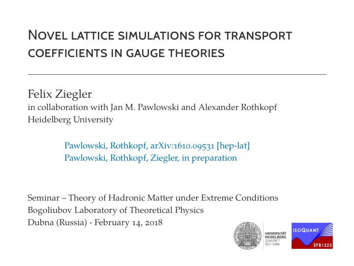
NOVEL LATTICE SIMULATIONS FOR TRANSPORT COEFFICIENTS IN GAUGE THEORIES Felix Ziegler in collaboration with Jan M. Pawlowski and Alexander Rothkopf Heidelberg University Pawlowski, Rothkopf, arXiv:1610.09531 [hep-lat] Pawlowski, Rothkopf, Ziegler, in preparation Seminar – Theory of Hadronic Matter under Extreme Conditions Bogoliubov Laboratory of Theoretical Physics Dubna (Russia) - February 14, 2018 ISO Q UANT SFB 1225

Overview � Introduction ◦ Physics motivation of real-time dynamics from lattice QCD ◦ Challenges in the reconstruction of spectral functions � Novel simulation approach for thermal fields on the lattice with non-compact Euclidean time ◦ Setup and scalar fields ◦ Gauge fields ◦ Convergence to the Matsubara results ◦ Energy-momentum tensor correlation functions ◦ Spectral reconstructions � Summary and outlook 1

INTRODUCTION

P hysics motivation � Thermal physics of hot strongly interacting matter produced in heavy ion collisions ◦ Transport phenomena ◦ In-medium modification of heavy bound states � Transport coefficients are real-time quantities related to the energy-momentum tensor (EMT) correlation function � Example: shear viscosity � d 4 x ρ ( ω, 0 ) 1 x �[ T 12 ( x ) , T 12 ( 0 )]� . ( 2 π ) 4 e − i ω x 0 + i � p · � ρ ( ω, � η � lim , p ) � 20 ω ω → 0 ⇒ need spectral function ρ ( ω, � p ) 3

Lattice QCD at finite temperature � Gauge fields on links U µ ( x ) � exp ( iga µ A a µ ( x ) T a ) � Dynamical fermions with realistic masses � finite extent in imaginary time 1 / T � β � N τ a τ x β � N τ a τ τ � � O ( U )� � 1 D U O ( U ) exp ( − S QCD [ U ]) E Z N cf 1 � P ( U k ) � e − S QCD [ U k ] ⇒ � O ( U )� ≈ O ( U k ) E N cf 4 k � 1

R econstruction of spectral functions and its challenges � Back to real-time EMT-correlator: � d 4 x x �[ T 12 ( x ) , T 12 ( 0 )]� ( 2 π ) 4 e − i ω x 0 + i � p · � ρ ( ω, � p ) � � Spectral function connects physical real-time observable with Euclidean time simulation � � d µ cosh [ µ ( τ − β/ 2 )] d 3 x � T 12 ( τ, � D ( τ ) ∝ x ) T 12 ( 0 , 0 )� � ρ ( µ ) sinh [ µ β/ 2 ] For the reconstruction technique used in the following see Y.Burnier, Alexander Rothkopf, Phys.Rev.Lett. 111 (2013) 182003 5

R econstruction of spectral functions and its challenges Two main conceptual problems of standard spectral reconstructions � Problem 1: � ∞ d µ cosh [ µ ( τ − β/ 2 )] D ( τ ) � ρ ( µ ) sinh [ µ β/ 2 ] 0 Extraction from imaginary time correlator ill-posed exponentially hard inversion problem. → Go to imaginary frequencies and use Källén-Lehman spectral representation � ∞ 2 µ D ( ω n ) � d µ n + µ 2 ρ ( µ ) ω 2 0 6

R econstruction of spectral functions and its challenges Two main conceptual problems of standard spectral reconstructions � Problem 2: Increasing the number of points along Euclidean time axis does not help! Most relevant regime for the inverse problem: ω∼ T=1/ β � Standard lattice simulations only access Matsubara frequencies ω n � 2 π Tn , n ∈ Z . 7

SETUP OF A NOVEL COMPUTATIONAL APPROACH

T hermal field theory on the Schwinger-Keldysh contour � Thermal scalar field theory as a real-time initial value problem with ρ ( 0 ) � e − β H � Z � Tr � � d [ ϕ + 0 ] d [ ϕ − 0 ]� ϕ + 0 | ρ ( 0 )| ϕ − 0 �� ϕ − 0 | ϕ + Z � 0 � initial conditions ρ (0)=e - β H t 9

T hermal field theory on the Schwinger-Keldysh contour � Thermal scalar field theory as a real-time initial value problem with ρ ( 0 ) � e − β H � Z � Tr � � � d [ ϕ + 0 ] d [ ϕ − 0 ]� ϕ + 0 | ρ ( 0 )| ϕ − 0 �� ϕ − 0 | ϕ + [ d ϕ t ]� ϕ − 0 | e iHt | ϕ t �� ϕ t | e − iHt | ϕ + Z � 0 � 0 � initial conditions quantum dynamics φ + (t) ρ (0)=e - β H φ - (t) t 10

T hermal field theory on the Schwinger-Keldysh contour � Thermal scalar field theory as a real-time initial value problem with ρ ( 0 ) � e − β H � Z � Tr � � ϕ − � 0 D ϕ e iS M [ ϕ + ] − iS M [ ϕ − ] d [ ϕ + 0 ] d [ ϕ − 0 ]� ϕ + 0 | e − β H | ϕ − 0 �� ϕ − 0 | ϕ + Z � 0 � ϕ + 0 initial conditions quantum dynamics φ + (t) ρ (0)=e - β H φ - (t) t 11

T hermal field theory on the Schwinger-Keldysh contour � Thermal scalar field theory as a real-time initial value problem with ρ ( 0 ) � e − β H � Z � Tr � � ϕ − ( t 0 ) � ϕ E ( β ) � D ϕ e iS M [ ϕ + ] − iS M [ ϕ − ] D ϕ E e − S E [ ϕ E ] Z � ϕ E ( 0 ) � ϕ E ( β ) ϕ + ( t 0 ) � ϕ E ( 0 ) initial conditions τ 0 =t 0 quantum dynamics φ + (t) φ E ( τ ) φ - (t) β =1/T t τ � So far, we have only rewritten the partition function. The imaginary time is a mathematical tool to sample initial conditions ϕ + ( t 0 ) and ϕ − ( t 0 ) . 12

P ath contribution � Thermal equilibrium ⇒ G ++ ≡ � ϕ + ϕ + � correlator sufficient to compute spectral function ρ , see e.g. Laine and Vuorinen, Basics of Thermal Field Theory, Springer 2016 � d q 0 ρ ( q 0 , � p ) G ++ ( p 0 , � q 0 − p 0 + i ε − n ( p 0 ) ρ ( p 0 , � p ) � p ) 2 π initial conditions τ 0 =t 0 quantum dynamics φ + (t) φ E ( τ ) φ - (t) β =1/T t τ � Using time translation invariance we can set t 0 → −∞ . � Introducing ε > 0 and e − iHt → e − iHt ( 1+ i ε ) correlations between any finite t on forward branch and endpoint become exponentially damped. 13

Analytic continuation and general imaginary frequencies � From no on, we focus on the forward ϕ + path. � Idea: Cut open real-time path at t � ∞ and rotate path to (additional) non-compact imaginary time axis. � ϕ − ( t 0 ,� � x ) � ϕ E ( β ) D ϕ e i S M [ ϕ + ] − i S M [ ϕ − ] D ϕ E e − S E [ ϕ E ] Z � ϕ E ( 0 ) � ϕ E ( β ) ϕ + ( t 0 ,� x ) � ϕ E ( 0 ) initial conditions τ 0 =t 0 quantum dynamics φ + (t) φ E ( τ ) φ - (t) β =1/T t τ 14

Analytic continuation and general imaginary frequencies � From no on, we focus on the forward ϕ + path. � Idea: Cut open real-time path at t � ∞ and rotate path to (additional) non-compact imaginary time axis. � ϕ + ( ∞ ) � ϕ − ( τ 0 ) � ϕ E ( β ) � D ϕ + e − S E [ ϕ + ] D ϕ E e − S E [ ϕ E ] D ϕ − e − S E [ ϕ − ] Z � ϕ E ( 0 ) � ϕ E ( β ) ϕ + ( τ 0 ) � ϕ E ( 0 ) ϕ − ( ∞ ) τ Simulation recipe φ + ( τ ) τ 0 = τ 0 =t 0 τ 0 ) � ϕ + ( τ 0 ) � Sample init. conditions ϕ E ( ¯ initial conditions from e − S E [ ϕ E ] on compact Euclidean quantum dynamics φ + (t) φ E ( τ ) time lattice, ¯ τ ∈ [ 0 , β ] . φ - (t) β =1/T t τ � Concurrently sample ϕ + ( τ ) from e − S E [ ϕ + ] with τ ∈ [ 0 , ∞ ) . 15

S imulating scalar fields � 1 � + λ 2 ( ∂ τ ϕ E ) 2 + 1 � 4! ϕ 4 2 m 2 ϕ 2 δ S E S E � d τ E E ∂ t 5 ϕ E ( ¯ τ k ) � − τ k ) + η ( ¯ τ k ) δϕ E ( ¯ � �������������������� �� �������������������� � ���� S 0 S int E E δ S 0 δ S int δϕ + ( τ j ) � Temperature in ϕ E via ∂ t 5 ϕ + ( ω l ) � − E E ϕ + ( ω l ) + η ( ω l ) δϕ + ( ω l ) − compact temporal path δϕ + ( τ j ) � Temperature in ϕ + via initial condition ϕ + ( t 0 ) � Use Stochastic Quantization and sample ϕ E and ϕ + concurrently from Langevin μ τ equations τ 0 = τ 0 = t 0 � Imaginary frequency update in Fourier Fourier analytic space continuation → kinetic term diagonal and improved 𝜒 E ( τ ) β =1/T t convergence τ quantum dynamics initial ¡conditions 16

NUMERICAL RESULTS FOR SCALAR FIELD THEORIES

0+1 dimensional real scalar field Two-point correlation function 0.32 0.004 λ =0 λ =24 0.3 0.002 N MB N MB ω =16 ω =16 ‾ ) φ E (0)> 0 10 G ++ ( ω )=< φ + ( ω ) φ + (- ω )> N ω =512 N ω =512 -0.002 0.28 Δ G/G QM vs. SQ N ω =256 N ω =256 -0.004 N ω =128 N ω =128 0 0.3 0.6 0.9 ‾ )=< φ E ( τ N ω =64 N ω =64 0.26 τ ‾ /m N ω =32 N ω =32 QM N ω =16 N ω =16 1 SQ N τ =128 0.24 N τ =64 G E ( τ N τ =32 Free x2 N τ =16 0.22 λ =24 0.2 0.1 0 0.2 0.4 0.6 0.8 1 0 2 4 6 8 10 12 14 τ ‾ /m ω /m Figure: Free and interacting theory Figure: QM (an-)harmonic oscillator from general frequency simulations vs. stoch. quantization result on the compact Euclidean time lattice Pawlowski, Rothkopf, arXiv:1610.09531 [hep-lat] 18

0+1 dimensional real scalar field Two-point correlation function 4.4 4.2 λ =0 λ =24 G ++ ( ω ) 4 N MB N MB ω =16 ω =16 10 3.8 G ++ ( ω )=< φ + ( ω ) φ + (- ω )> N ω =512 N ω =512 3.6 N ω =256 N ω =256 3.4 N ω =128 N ω =128 3.2 N ω =64 N ω =64 0 0.2 0.4 0.6 0.8 1 N ω =32 N ω =32 ω /m N ω =16 N ω =16 1 (G imag -G mats )/G mats 0.035 0.03 N Free ω =16 N ω =16 Free x2 0.025 0.02 0.015 0.01 0.005 0.1 0 -0.005 0 2 4 6 8 10 12 14 0 10 20 30 40 50 ω /m ω /m Convergence properties of the correlator 19