Not Too Different From Discrete... A Note on Independence For - PowerPoint PPT Presentation

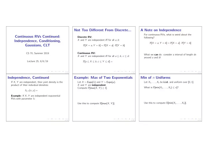
Not Too Different From Discrete... A Note on Independence For continuous RVs, what is weird about the Continuous RVs Continued: Discrete RV: following? X and Y are independent iff for all a , b : Independence, Conditioning, P [ X = a , Y = b ] = P [ X = a ] · P [ Y = b ] Gaussians, CLT P [ X = a , Y = b ] = P [ X = a ] · P [ Y = b ] Continuous RV: CS 70, Summer 2019 What we can do: consider a interval of length dx X and Y are independent iff for all a ≤ b , c ≤ d : around a and b ! Lecture 25, 8/6/19 P [ a ≤ X ≤ b , c ≤ Y ≤ d ] = 1 / 26 2 / 26 3 / 26 Independence, Continued Example: Max of Two Exponentials Min of n Uniforms If X , Y are independent, their joint density is the Let X ∼ Expo( λ ) and Y ∼ Expo( µ ) . Let X 1 , . . . , X n be i.i.d. and uniform over [ 0 , 1 ] . product of their individual densities: X and Y are independent . What is P [min( X 1 , . . . , X n ) ≤ x ] ? Compute P [max( X , Y ) ≥ t ] . f X , Y ( x , y ) = Example: If X , Y are independent exponential RVs with parameter λ : Use this to compute E [min( X 1 , . . . , X n )] . Use this to compute E [max( X , Y )] . 4 / 26 5 / 26 6 / 26

Min of n Uniforms Memorylessness of Exponential Conditional Density We can’t talk about independence without talking What happens if we condition on events like What is the CDF of min( X 1 , . . . , X n ) ? about conditional probability ! X = a ? These have 0 probability! Let X ∼ Expo( λ ) . X is memoryless , i.e. The same story as discrete, except we now need to define a conditional density : What is the PDF of min( X 1 , . . . , X n ) ? P [ X ≥ s + t | X > t ] = P [ X ≥ s ] f Y | X ( y | x ) = f X , Y ( x , y ) f X ( x ) Think of f ( y | x ) as P [ Y ∈ [ y , y + dy ] | X ∈ [ x , x + dx ]] 7 / 26 8 / 26 9 / 26 Conditional Density, Continued Example: Sum of Two Exponentials Example: Total Probability Rule Given a conditional density f Y | X , compute Let X 1 , X 2 be i.i.d Expo( λ ) RVs. What is the CDF of Y ? Let Y = X 1 + X 2 . P [ Y ≤ y | X = x ] = What is P [ Y < y | X 1 = x ] ? What is the PDF of Y ? If we know P [ Y ≤ y | X = x ] , compute What is P [ Y < y ] ? P [ Y ≤ y ] = Go with your gut! What worked for discrete also works for continuous. 10 / 26 11 / 26 12 / 26

Break The Normal (Gaussian) Distribution Gaussian Tail Bound Let X ∼ N ( 0 , 1 ) . X is a normal or Gaussian RV if: Easy upper bound on P [ | X | ≥ α ] , for α ≥ 1? 1 2 πσ 2 · e − ( x − µ ) 2 / 2 σ 2 √ (Something we’ve seen before...) f X ( x ) = If you could immediately gain one new skill, what Parameters: would it be? Notation: X ∼ E [ X ] = Var( X ) = Standard Normal: 13 / 26 14 / 26 15 / 26 Gaussian Tail Bound, Continued Shifting and Scaling Gaussians Shifting and Scaling Gaussians Let X ∼ N ( µ, σ ) and Y = X − µ Turns out we can do better than Chebyshev. σ . Then: Can also go the other direction: � ∞ 2 π e − x 2 / 2 dx ≤ 1 Idea: Use Y ∼ If X ∼ N ( 0 , 1 ) , and Y = µ + σ X : √ α Y is still Gaussian! Proof: Compute P [ a ≤ Y ≤ b ] . E [ Y ] = Var( Y ) = Change of variables: x = σ y + µ . 16 / 26 17 / 26 18 / 26

Sum of Independent Gaussians Example: Height Example: Height Let X , Y be independent standard Gaussians. Consider a family of a two parents and twins with the same height. The parents’ heights are E [ H ] = Let Z = [ aX + c ] + [ bY + d ] . independently drawn from a N ( 65 , 5 ) distribution. Then, Z is also Gaussian! (Proof optional.) The twins’ height are independent of the parents’, and from a N ( 40 , 10 ) distribution. E [ Z ] = Let H be the sum of the heights in the family. Define relevant RVs: Var[ H ] = Var( Z ) = 19 / 26 20 / 26 21 / 26 Sample Mean The Central Limit Theorem (CLT) Example: Chebyshev vs. CLT We sample a RV X independently n times. Let X 1 , X 2 , . . . , X n be i.i.d. RVs with mean µ , Let X 1 , X 2 , . . . be i.i.d RVs with E [ X i ] = 1 and X has mean µ , variance σ 2 . variance σ 2 . (Assume mean, variance, are finite.) Var( X i ) = 1 2 . Let A n = X 1 + X 2 + ... + X n . n Denote the sample mean by A n = X 1 + X 2 + ... + X n Sample mean, as before: A n = X 1 + X 2 + ... + X n E [ A n ] = n n Recall: E [ A n ] = E [ X ] = Var( A n ) = Var( A n ) = Normalize the sample mean: Normalize to get A ′ Var( X ) = n : A ′ n = Then, as n → ∞ , P [ A ′ n ] → 22 / 26 23 / 26 24 / 26

Example: Chebyshev vs. CLT Summary Upper bound P [ A ′ n ≥ 2 ] for any n . ◮ Independence and conditioning also (We don’t know if A ′ n is non-neg or symmetric .) generalize from the discrete RV case. ◮ The Gaussian is a very important continuous RV. It has several nice properties, including the fact that adding independent Gaussians If we take n → ∞ , upper bound on P [ A ′ n ≥ 2 ] ? gets you another Gaussian ◮ The CLT tells us that if we take a sample average of a RV, the distribution of this average will approach a standard normal . 25 / 26 26 / 26