Nonlinear Planetary Wave Dynamics of Quasi-Stationary Anomalies - PowerPoint PPT Presentation

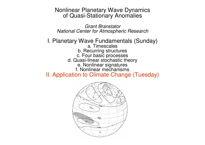
Nonlinear Planetary Wave Dynamics of Quasi-Stationary Anomalies Grant Branstator National Center for Atmospheric Research I. Planetary Wave Fundamentals (Sunday) a. Timescales b. Recurring structures c. Four basic processes d. Quasi-linear stochastic theory e. Nonlinear signatures f. Nonlinear mechanisms II. Application to Climate Change (Tuesday)

January 300mb psi high/positive low/negative

January 300mb psi

h500 Average temporal spectrum T31 LFV Transient eddies

Psi300 zonal wavenumber spectra for Nature LFV synoptic 2 4 6 8 10 12 14 Zonal wave number

Psi300 zonal wavenumber spectra for Nature barotropic LFV synoptic baroclinic 2 4 6 8 10 12 14 Zonal wave number

psi300 x “Teleconnection Patterns” x

h500 EOFs Most predictable patterns for 10d forecasts

El Nino composite h500 anomalies 1958,1966,1973,1983,1987,1992

Low frequency perturbations are: 1. Large-scale 2. On a rotating planet 3. Barotropic 4. Non-divergent in the upper tropospheric midlatitudes 5. Relatively weak compared to time mean state Therefore: Linear, barotropic vorticity dynamics should be important for understanding their behavior.

Basic quasi-linear barotropic dynamics ∂ς ∂ t = − r ψ ⋅ ∇ ( ς + f ) v 2 Ω sin ϕ T ∫ ( • ) = 1 ( • ) dt + ( • )' = () + ( • )' T 0 ∂ς ' = − r ψ ⋅ ∇ ( ς + f ) − r ψ ⋅ ∇ς ' − r ψ ⋅∇ ( ς + f ) − r ψ ⋅∇ς ' v v v ' v ' ∂ t r ψ ⋅ ∇ ( ς + f ) = − r ψ ⋅∇ς ' v v ' ∂ς ' = − r ψ ⋅ ∇ς ' − r ψ ⋅∇ ( ς + f ) − ( r ψ ⋅∇ς ' − r ψ ⋅∇ς ' ) ' ' ' v v v v ∂ t ∂ ′ ς * − r # •∇ ′ ς − r ς − r ∂ t = − [ u ] ′ ς x − ′ v β v •∇ ′ ′ v •∇ ′ ′ ς ∂ς ' v ∂ t ≅ − r ψ ⋅ ∇ς ' − r ψ ⋅∇ ( ς + f ) + damping + noise v v ' I II III IV

Linear Initial Value Problem Using Normal Mode Basis ∂ ′ ς ∂ t = − r ς − r ψ ⋅∇ ′ ψ ⋅∇ ( ς + f ) ′ v v = L ′ ς Say LE = σ E σ t = ( E R + iE I ) e σ R t (cos σ I t + i sin σ I t ) Then ′ ς ( t ) = Ee = e σ R t { E R cos σ I t − E I sin σ I t } + i {...} is a solution. ∑ Thus, if ′ ς ( t = 0) = j is real, a j E j ∑ j t { j cos σ I j sin σ I then ′ ς (t) = j t − E I σ R j t } a j e E R j

For solid body rotation background u = u e cos ϕ ′ ′ ∂ ς ∂ ς * 1 1 d f ′ = − − ( ) ( ) u v ψ ∂ ∂ λ ϕ e t a a d m Y Normal modes are spherical harmonics n with frequency   2 Ω * σ I = u a −   e m n ( n + 1)  

Wallace and Lau (1985) … ′ ′ ∂ ∂ < + > ∂ ∂ 2 2 KE ( u v ) u u ′ ′ ′ ′ = = − < − > − < >= + 2 2 ( u v ) u v CKx CKy ∂ ∂ ∂ ∂ t t x y

Mean Jan 300mb Psi Linear Vorticity Equation

Linear Vorticity Equation

(Branstator, 1985) (Simmons et al., 1983)

Fastest Growing Normal Mode (Simmons et al., 1983)

Basic linear barotropic stochastic dynamics ∂ς ∂ t = − r ψ ⋅ ∇ ( ς + f ) v T ∫ ( • ) = 1 ( • ) dt + ( • )' = () + ( • )' T 0 ∂ς ' = − r ψ ⋅ ∇ ( ς + f ) − r ψ ⋅ ∇ς ' − r ψ ⋅∇ ( ς + f ) − r ψ ⋅∇ς ' v v v ' v ' ∂ t r ψ ⋅ ∇ ( ς + f ) = − r ψ ⋅∇ς ' v v ' ∂ς ' = − r ψ ⋅ ∇ς ' − r ψ ⋅∇ ( ς + f ) − ( r ψ ⋅∇ς ' − r ψ ⋅∇ς ' ) v v ' v ' v ' ∂ t ∂ς ' ∂ t ≅ − r ψ ⋅ ∇ς ' − r ψ ⋅∇ ( ς + f ) + damping + noise v v ' (Dymnikov, 1988)

Stochastically Driven Linear Barotropic Vorticity Equation Variance

Stochastically Driven Linear Barotropic Vorticity Equation Variance

Linear Stochastic Model of Planetary Waves ∂ ′ ς ∂ t = − r ς − r v •∇ ′ v •∇ ( ς + f ) + damping + Gaussian noise ′ Signatures of linear behavior: � Gaussian PDFs � Elliptical trajectories

Projections onto EOF1&2 Low pass winter h500 EOFs PDF G A R Cheng & Wallace (1992)

10d means from 7,500,000d 10d means from 5000d sample sample Berner & Branstator

Slices through AGCM phase space Berner & Branstator (2007)

Branstator & Berner (2005)

Mean 24hr increments Branstator & Berner (2005)

Branstator & Berner (2005)

∂ς ' = − r ψ ⋅ ∇ς ' − r ψ ⋅∇ ( ς + f ) − ( r ψ ⋅∇ς ' − r ψ ⋅∇ς ' ) v v ' v ' v ' ∂ t ∂ς ∂ t

Multiple Equilibria following Charney & Devore (1979) and Held (1983) ∂ [ u ] ∂ t = −κ ([ u ] − [ u e ]) − D ([ u ]) for D([u]) = ∂ * ∂ h t * ] + 1 * v ∂ y[ u [ p ∂ x ] h 0 C D ([ u ]) −κ ([ u ] − [ u e ]) A

PDF Lorenz63 = − σ + σ & X X Y = − + − & Y XZ rX Y = − & Z XY bZ

h500 Average temporal spectrum T31 LFV Transient eddies

− 5 2 1 100 10 x m s − − 2 2 13 4 2 2 x 10 m s 5 m s

Linear Stormtrack Model ∂ ς ' r r ′ = − ⋅ ∇ ς − ⋅∇ ς + + v v ' ... damping ∂ t ∂ T ' r r = − ⋅ ∇ − ⋅∇ + + v T ' v ' T ... damping ∂ t ∂ D ' = ... ∂ t ∂ p = s ... ∂ t

Psi300 NAO+ NAO-

∂ ς r = − ⋅ ∇ ς + − v ( f ) ... ψ ∂ t T 1 ∫ ′ = + () () dt ( ) T 0 ′ ∂ ς r r r r ′ = − ⋅ ∇ ς + − ⋅ ∇ ς − ⋅∇ ς − ⋅∇ ς v ( f ) v v ' v ' '... ψ ψ ψ ψ ∂ t r r ⋅ ∇ ς + = − ⋅∇ ς + v ( f ) v ' ' ... ψ ψ ′ ∂ ς r r r r ′ = − ⋅ ∇ ς − ⋅∇ ς − ⋅∇ ς − ⋅∇ ς v v ' ( v ' ' v ' ' )... ψ ψ ψ ψ ∂ t r r ′ = − ⋅ ∇ ς − ⋅∇ ς + + v v ' damping noise ... T ′ ψ ψ ς

E=14.8d E=5.6d

LinBaroVorEqn + CCM0 LinBaroVorEqn TranEddyFeedbk 18% 21% 36%

Nonlinear Planetary Wave Dynamics of Quasi-Stationary Anomalies Grant Branstator National Center for Atmospheric Research I. Planetary Wave Fundamentals (Sunday) a. Timescales b. Recurring structures c. Four basic processes d. Quasi-linear stochastic theory e. Nonlinear signatures f. Nonlinear mechanisms II. Application to Climate Change (Tuesday)