Non-Gaussianity as a Probe of the Physics of the Primordial - PowerPoint PPT Presentation

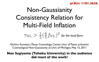
Non-Gaussianity as a Probe of the Physics of the Primordial Universe Eiichiro Komatsu (Texas Cosmology Center, University of Texas at Austin) Solvary Workshop, “Cosmological Frontiers in Fundamental Physics” May 13, 2009 1

How Do We Test Inflation? • How can we answer a simple question like this: • “ How were primordial fluctuations generated? ” 2

Power Spectrum • A very successful explanation (Mukhanov & Chibisov; Guth & Pi; Hawking; Starobinsky; Bardeen, Steinhardt & Turner) is: • Primordial fluctuations were generated by quantum fluctuations of the scalar field that drove inflation. • The prediction: a nearly scale-invariant power spectrum in the curvature perturbation, ζ : • P ζ (k) = A/k 4–ns ~ A/k 3 • where n s ~1 and A is a normalization. 3

Komatsu et al. (2009) n s <1 Observed • The latest results from the WMAP 5-year data: • n s =0.960 ± 0.013 (68%CL; for tensor modes = zero) • n s =0.970 ± 0.015 (68%CL; for tensor modes ≠ zero) • tensor-to-scalar ratio < 0.22 (95%CL) • n s ≠ 1: another line of evidence for inflation • Detection of non-zero tensor modes is a next important step 4

Anything Else? • One can also look for other signatures of inflation. For example: • Isocurvature perturbations • Proof of the existence of multiple fields • Non-zero spatial curvature • Evidence for “Landscape,” if curvature is negative. Rules out Landscape ideas if positive. • Scale-dependent n s (running index) • Complex dynamics of inflation 5

Komatsu et al. (2009) Anything Else? • One can also look for other signatures of inflation. For example: • 95%CL limits on Isocurvature perturbations • S/(3 ζ ) <0.089 (axion CDM); <0.021 (curvaton CDM) • 95%CL limits on Non-zero spatial curvature • Ω –1<0.018 (for Ω >1); 1– Ω <0.008 (for Ω <1) positive curvature negative curvature • 95%CL limits on Scale-dependent n s • –0.068 < dn s /dlnk < 0.012 6

Beyond Power Spectrum • All of these are based upon fitting the observed power spectrum. • Is there any information one can obtain, beyond the power spectrum? 7

Bispectrum k 3 k 1 • Three-point function! k 2 • B ζ ( k 1 , k 2 , k 3 ) = < ζ k 1 ζ k 2 ζ k 3 > = (amplitude) x (2 π ) 3 δ ( k 1 + k 2 + k 3 )b(k 1 ,k 2 ,k 3 ) model-dependent function 8

Why Study Bispectrum? • It probes the interactions of fields - new piece of information that cannot be probed by the power spectrum • But, above all, it provides us with a critical test of the simplest models of inflation: “ are primordial fluctuations Gaussian, or non-Gaussian? ” • Bispectrum vanishes for Gaussian fluctuations. • Detection of the bispectrum = detection of non- Gaussian fluctuations 10

Gaussian? WMAP5 11

Spergel et al. (2008) Take One-point Distribution Function •The one-point distribution of WMAP map looks pretty Gaussian. –Left to right: Q (41GHz), V (61GHz), W (94GHz). •Deviation from Gaussianity is small, if any. 12

Inflation Likes This Result • According to inflation (Mukhanov & Chibisov; Guth & Yi; Hawking; Starobinsky; Bardeen, Steinhardt & Turner), CMB anisotropy was created from quantum fluctuations of a scalar field in Bunch-Davies vacuum during inflation • Successful inflation (with the expansion factor more than e 60 ) demands the scalar field be almost interaction-free • The wave function of free fields in the ground state is a Gaussian! 13

But, Not Exactly Gaussian • Of course, there are always corrections to the simplest statement like this. • For one, inflaton field does have interactions. They are simply weak – they are suppressed by the so-called slow-roll parameter, ε ~O(0.01), relative to the free-field action. 14

A Non-linear Correction to Temperature Anisotropy • The CMB temperature anisotropy, Δ T/T, is given by the curvature perturbation in the matter-dominated era, Φ . • One large scales (the Sachs-Wolfe limit), Δ T/T=– Φ /3. For the Schwarzschild • Add a non-linear correction to Φ : metric, Φ =+GM/R. • Φ ( x ) = Φ g ( x ) + f NL [ Φ g ( x )] 2 (Komatsu & Spergel 2001) • f NL was predicted to be small (~0.01) for slow-roll models (Salopek & Bond 1990; Gangui et al. 1994) 15

f NL : Form of B ζ • Φ is related to the primordial curvature perturbation, ζ , as Φ =(3/5) ζ . • ζ ( x ) = ζ g ( x ) + (3/5)f NL [ ζ g ( x )] 2 • B ζ ( k 1 , k 2 , k 3 )=(6/5)f NL x (2 π ) 3 δ ( k 1 + k 2 + k 3 ) x [P ζ (k 1 )P ζ (k 2 ) + P ζ (k 2 )P ζ (k 3 ) + P ζ (k 3 )P ζ (k 1 )] 16

f NL : Shape of Triangle • For a scale-invariant spectrum, P ζ (k)=A/k 3 , • B ζ ( k 1 , k 2 , k 3 )=(6A 2 /5)f NL x (2 π ) 3 δ ( k 1 + k 2 + k 3 ) x [1/(k 1 k 2 ) 3 + 1/(k 2 k 3 ) 3 + 1/(k 3 k 1 ) 3 ] • Let’s order k i such that k 3 ≤ k 2 ≤ k 1 . For a given k 1 , one finds the largest bispectrum when the smallest k, i.e., k 3 , is very small. • B ζ ( k 1 , k 2 , k 3 ) peaks when k 3 << k 2 ~k 1 • Therefore, the shape of f NL bispectrum is the squeezed triangle! (Babich et al. 2004) 17

B ζ in the Squeezed Limit • In the squeezed limit, the f NL bispectrum becomes: B ζ ( k 1 , k 2 , k 3 ) ≈ (12/5)f NL x (2 π ) 3 δ ( k 1 + k 2 + k 3 ) x P ζ (k 1 )P ζ (k 3 ) 18

Maldacena (2003); Seery & Lidsey (2005); Creminelli & Zaldarriaga (2004) Single-field Theorem (Consistency Relation) • For ANY single-field models * , the bispectrum in the squeezed limit is given by • B ζ ( k 1 , k 2 , k 3 ) ≈ (1–n s ) x (2 π ) 3 δ ( k 1 + k 2 + k 3 ) x P ζ (k 1 )P ζ (k 3 ) • Therefore, all single-field models predict f NL ≈ (5/12)(1–n s ). • With the current limit n s =0.96, f NL is predicted to be 0.017. * for which the single field is solely responsible for driving inflation and generating observed fluctuations. 19

Understanding the Theorem • First, the squeezed triangle correlates one very long- wavelength mode, k L (=k 3 ), to two shorter wavelength modes, k S (=k 1 ≈ k 2 ): • < ζ k 1 ζ k 2 ζ k 3 > ≈ <( ζ k S ) 2 ζ k L > • Then, the question is: “why should ( ζ k S ) 2 ever care about ζ k L ?” • The theorem says, “it doesn’t care, if ζ k is exactly scale invariant.” 20

ζ k L rescales coordinates Separated by more than H -1 • The long-wavelength curvature perturbation rescales the spatial coordinates (or changes the expansion factor) within a given Hubble patch: • ds 2 =–dt 2 +[ a (t)] 2 e 2 ζ (d x ) 2 x 1 = x 0 e ζ 1 x 2 = x 0 e ζ 2 ζ k L 21 left the horizon already

ζ k L rescales coordinates Separated by more than H -1 • Now, let’s put small-scale perturbations in. • Q. How would the ( ζ k S1 ) 2 ( ζ k S2 ) 2 conformal rescaling of coordinates change the amplitude of the small-scale perturbation? x 1 = x 0 e ζ 1 x 2 = x 0 e ζ 2 ζ k L 22 left the horizon already

ζ k L rescales coordinates Separated by more than H -1 • Q. How would the conformal rescaling of coordinates change the amplitude of the small-scale ( ζ k S1 ) 2 ( ζ k S2 ) 2 perturbation? • A. No change, if ζ k is scale- invariant . In this case, no correlation between ζ k L and x 1 = x 0 e ζ 1 x 2 = x 0 e ζ 2 ( ζ k S ) 2 would arise. ζ k L 23 left the horizon already

Creminelli & Zaldarriaga (2004); Cheung et al. (2008) Real-space Proof • The 2-point correlation function of short-wavelength modes, ξ =< ζ S ( x ) ζ S ( y )>, within a given Hubble patch can be written in terms of its vacuum expectation value (in the absence of ζ L ), ξ 0 , as: • ξ ζ L ≈ ξ 0 (| x – y |) + ζ L [d ξ 0 (| x – y |)/d ζ L ] • ξ ζ L ≈ ξ 0 (| x – y |) + ζ L [d ξ 0 (| x – y |)/dln| x – y |] • ζ S ( y ) • ξ ζ L ≈ ξ 0 (| x – y |) + ζ L (1–n s ) ξ 0 (| x – y |) • ζ S ( x ) 3-pt func. = <( ζ S ) 2 ζ L > = < ξ ζ L ζ L > = (1–n s ) ξ 0 (| x – y |)< ζ L2 > 24

Where was “Single-field”? • Where did we assume “single-field” in the proof? • For this proof to work, it is crucial that there is only one dynamical degree of freedom, i.e., it is only ζ L that modifies the amplitude of short-wavelength modes, and nothing else modifies it. • Also, ζ must be constant outside of the horizon (otherwise anything can happen afterwards). This is also the case for single-field inflation models. 25

Therefore... • A convincing detection of f NL > 1 would rule out all of the single-field inflation models, regardless of: • the form of potential • the form of kinetic term (or sound speed) • the initial vacuum state • A convincing detection of f NL would be a breakthrough. 26

Large Non-Gaussianity from Single-field Inflation • S=(1/2) ∫ d 4 x √ –g [R–( ∂ μ φ ) 2 –2V( φ )] • 2nd-order (which gives P ζ ) • S 2 = ∫ d 4 x ε [ a 3 ( ∂ t ζ ) 2 – a ( ∂ i ζ ) 2 ] • 3rd-order (which gives B ζ ) • S 3 = ∫ d 4 x ε 2 [… a 3 ( ∂ t ζ ) 2 ζ +… a ( ∂ i ζ ) 2 ζ +… a 3 ( ∂ t ζ ) 3 ] + O( ε 3 ) Cubic-order interactions are suppressed by an additional factor of ε . (Maldacena 2003) 27