Non-Gaussianity Consistency Relation for Multi-Field Inflation for - PowerPoint PPT Presentation

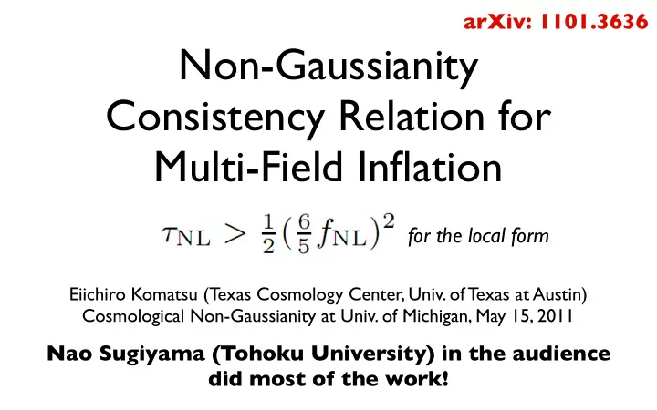
arXiv: 1101.3636 Non-Gaussianity Consistency Relation for Multi-Field Inflation for the local form Eiichiro Komatsu (Texas Cosmology Center, Univ. of Texas at Austin) Cosmological Non-Gaussianity at Univ. of Michigan, May 15, 2011 Nao Sugiyama (Tohoku University) in the audience did most of the work!

Theme • How to falsify inflation? or • Why bother measuring the trispectrum? 2

Motivation • I will be focused on the local-form non-Gaussianity. • The local-form bispectrum is particularly important because its detection would rule out all single-field inflation models (Creminelli & Zaldarriaga 2004). • f NLlocal >> 1 (like 30, as suggested by the current data) ALL single-field inflation models would be ruled out. But, what about multi-field models? 3

Motivation • Can we rule out multi-field models also? • If we rule out single-field AND multi-field, then... 4

Falsifying “inflation” • We still need inflation to explain the flatness problem! • (Homogeneity problem can be explained by a bubble nucleation.) • However, the observed fluctuations may come from different sources. • So, what I ask is, “can we rule out inflation as a mechanism for generating the observed fluctuations?” 5

Conclusion • It is almost possible. 6

Sugiyama, Komatsu & Futamase, arXiv: 1101.3636 Strategy • We look at the local-form four-point function (trispectrum). • Specifically, we look for a consistency relation between the local-form bispectrum and trispectrum that is respected by (almost) all models of multi-field inflation. • We found one: provided that 2-loop and higher-order terms are ignored. 7

Which Local-form Trispectrum? • The local-form bispectrum: • Β ζ ( k 1 , k 2 , k 3 ) =(2 π ) 3 δ ( k 1 + k 2 + k 3 )f NL [(6/5)P ζ (k 1 )P ζ (k 2 )+cyc.] • can be produced by a curvature perturbation in position space in the form of: • ζ ( x )= ζ g ( x ) + (3/5)f NL [ ζ g ( x )] 2 • This can be extended to higher-order: • ζ ( x )= ζ g ( x ) + (3/5)f NL [ ζ g ( x )] 2 + (9/25)g NL [ ζ g ( x )] 3 This term ( ζ 3 ) is too small to see, so I will ignore this in this talk. 8

Two Local-form Shapes • For ζ ( x )= ζ g ( x ) + (3/5)f NL [ ζ g ( x )] 2 + (9/25)g NL [ ζ g ( x )] 3 , we obtain the trispectrum: • T ζ ( k 1 , k 2 , k 3 , k 4 )=(2 π ) 3 δ ( k 1 + k 2 + k 3 + k 4 ) { g NL [(54/25)P ζ (k 1 ) P ζ (k 2 )P ζ (k 3 )+cyc.] + (f NL ) 2 [(18/25)P ζ (k 1 )P ζ (k 2 )(P ζ (| k 1 + k 3 |) +P ζ (| k 1 + k 4 |))+cyc.]} k 2 k 3 k 2 k 3 k 4 k 1 k 4 k 1 g NL f NL2 9

Generalized Trispectrum • T ζ ( k 1 , k 2 , k 3 , k 4 )=(2 π ) 3 δ ( k 1 + k 2 + k 3 + k 4 ) { g NL [(54/25) P ζ (k 1 )P ζ (k 2 )P ζ (k 3 )+cyc.] + τ NL [P ζ (k 1 )P ζ (k 2 )(P ζ (| k 1 + k 3 |)+P ζ (| k 1 + k 4 |))+cyc.]} The single-source local form consistency relation, τ NL =(6/5)(f NL ) 2 , may not be respected – additional test of multi-field inflation! k 2 k 3 k 2 k 3 k 4 k 1 k 4 k 1 g NL τ NL 10

(Slightly) Generalized Trispectrum • T ζ ( k 1 , k 2 , k 3 , k 4 )=(2 π ) 3 δ ( k 1 + k 2 + k 3 + k 4 ) { g NL [(54/25) P ζ (k 1 )P ζ (k 2 )P ζ (k 3 )+cyc.] + τ NL [P ζ (k 1 )P ζ (k 2 )(P ζ (| k 1 + k 3 |)+P ζ (| k 1 + k 4 |))+cyc.]} The single-source local form consistency relation, τ NL =(6/5)(f NL ) 2 , may not be respected – additional test of multi-field inflation! k 2 k 3 k 2 k 3 k 4 k 1 k 4 k 1 g NL τ NL 11

Tree-level Result (Suyama & Yamaguchi) • Usual δ N expansion to the second order gives: 12

Now, stare at these. 13

Change the variable... (6/5)f NL = ∑ I a I b I τ NL =( ∑ I a I2 )( ∑ I b I2 ) 14

Then apply the Cauchy-Schwarz Inequality • Implies (Suyama & Yamaguchi 2008) But, this is valid only at the tree level! 15

Harmless models can violate the tree-level result • The Suyama-Yamaguchi inequality does not always hold because the Cauchy-Schwarz inequality can be 0=0. For example: In this harmless two-field case, the Cauchy-Schwarz inequality becomes 0=0 (both f NL and τ NL result from the second term). In this case, (Suyama & Takahashi 2008) 16

“1 Loop” Fourier transform this, and multiply 3 times p min =1/L • k b =min(k 1 ,k 2 ,k 3 ) 17

Assumptions • Scalar fields are responsible for generating fluctuations. • Fluctuations are Gaussian and scale-invariant at the horizon crossing. • All (local-form) non-Gaussianity was generated outside the horizon by δ N 18

Starting point • We need the fourth-order expansion for the complete calculation at the 1-loop level. • Then, Fourier transform this and calculate the bispectrum and trispectrum... 19

where [Byrnes et al. (2007)] where 20

21

22

1st term • where we have used the Cauchy-Schwarz inequality: ( ∑ a u a v a ) 2 ≤ ( ∑ a u a 2 )( ∑ a v a 2 )

24

2nd term • where we have used the Cauchy-Schwarz inequality: with • and 25

Sugiyama, Komatsu & Futamase, arXiv:1101.3636 Collecting terms, here comes a simple result • where (2 loop) denotes the following particular term: (2 loop) = 26

Now, ignore this 2-loop term: • The effect of including all 1-loop terms is to change the coefficient of Suyama-Yamaguchi inequality, τ NL ≥ (6f NL /5) 2 • This relation can have a logarithmic scale dependence. 27

What we have learned • The tree-level inequality cannot be taken at the face value. • 1-loop corrections do not destroy the inequality completely (it just modifies the coefficient), so it can still be used to falsify inflation as a mechanism for generating the observed fluctuations. 28

Implications for Inflation 4-point amplitude ln( τ NL ) • The current limits 3.3x10 4 from WMAP 7-year (Smidt et are consistent with al. 2010) single-field or multi- field models. • So, let’s play around with the future. 3-point ln(f NL ) 74 amplitude 29 (Komatsu et al. 2011)

Case A: Single-field Happiness ln( τ NL ) • No detection of anything (f NL or τ NL ) after Planck. Single-field survived the test (for the moment: the future galaxy surveys can 600 improve the limits by a factor of ten). ln(f NL ) 10 30

(Suyama & Yamaguchi 2008; Komatsu 2010; Sugiyama, Komatsu & Futamase 2011) Case B: Multi-field Happiness(?) ln( τ NL ) • f NL is detected. Single-field is gone. • But, τ NL is also detected, in accordance with τ NL >0.5(6f NL /5) 2 expected from most 600 multi-field models. ln(f NL ) 30 31

(Suyama & Yamaguchi 2008; Komatsu 2010; Sugiyama, Komatsu & Futamase 2011) Case C: Madness • f NL is detected. Single- ln( τ NL ) field is gone. • But, τ NL is not detected, or found to be negative , inconsistent Remember: with τ NL >0.5(6f NL /5) 2 . τ NL is not positive definite • Single-field AND 600 most of multi-field models are gone. ln(f NL ) 30 32