New concepts emerging from a linear response theory for - PowerPoint PPT Presentation
New concepts emerging from a linear response theory for nonequilibrium Marco Baiesi Physics and Astronomy Department Galileo Galilei, University of Padova, and INFN in co lm aboration with Christian Maes, Urna Basu,
New concepts emerging from a linear response theory for nonequilibrium Marco Baiesi � Physics and Astronomy Department “Galileo Galilei”, � University of Padova, and INFN � � in co lm aboration with Christian Maes, Urna Basu, � Eugenio Lippie lm o, Alessandro Sarracino, Bram Wynants, Eliran Boksenbojm GGI Workshop, 26-30 May, 2014
Overview Linear response � Linear response to temperature kicks � Entropy production and something else � Time-symmetric quantities: how many?
A macroscopic FPU? Livia Conti, Lamberto Rondoni, et al: www.rarenoise.lnl.infn.it
Linear response for FPU? How does a Fermi-Pasta-Ulam chain react to a change in one temperature? � Nonequilibrium specific heat variance of the energy � 6 = Compressibility in nonequilibrium?
Fluctuation-Dissipation Th.: Kubo � d h A ( t ) i = 1 d ds h A ( t ) V ( s ) i E → E − h s V dh s T An observable A(t) reacts to the appearance of a potential V(s) � 1 d is the entropy production from -V dsV ( s ) T
Out of equilibrium: many FDT a1) perturb the density of states and evolve (Agarwal, Vulpiani & C, Seifert & Speck, Parrondo &C,…) � a2) “bring back” the observable to the perturbation (Ruelle) � b) probability of paths (Cugliandolo &C, Harada- Sasa, Lippiello &C, Ricci-Tersenghi, Chatelain, Maes, …) � short review: Baiesi & Maes, New J. Phys. (2013)
Path probability (Markov), ω → { x s } for 0 ≤ s ≤ t Overdamped Langevin � p dx s = µ F ( s ) ds + 2 µT dB s � Discrete states C, C’, …with jump rates W ( C → C 0 )
Diffusion Probability of a sequence dx 0 , dx 1 , dx 2 , . . . ⇢ ( dB i ) 2 � dP i = (2 π dt ) − 1 / 2 exp 2 dt ⇢ [ dx i − µF ( i )] 2 � = (4 π µTdt ) − 1 / 2 exp 4 µTdt P ( ω ) = lim dt → 0 Π i dP i
Diffusion + perturbation dx s = µ F ( s ) ds + h s µ ∂ V p ∂ x ( s ) ds + 2 µT dB s Perturbation changes the path probability � Ratio of path probabilities is finite for dt → 0 P h ( ω ) P ( ω )
Susceptibility (h>0 for s>0) Generator ⇢ h Z t P h ( ω ) � 2 T [ V ( t ) − V (0)] − h P ( ω ) = exp LV ( s ) ds 2 T 0 P h ( ω ) ⌧ �� h A ( t ) i h � h A ( t ) i = A ( t ) P ( ω ) � 1 Susceptibility h A ( t ) i h � h A ( t ) i χ AV ( t ) = lim h h → 0
Markov generator ∂ x + µT ∂ 2 L = µF ∂ In this case: ∂ x 2 h LV i = d dt h V i interpret as expected variation: �� ⌧ dV � LV ( x ) = � dt � x
Response function Z t χ AV ( t ) = R AV ( t, s ) ds 0 d � R AV ( t, s ) = 1 ds h V ( s ) A ( t ) i � h LV ( s ) A ( t ) i 2 T 1/2 entropy production � minus 1/2 “expected” entropy production
Response function Z t χ AV ( t ) = R AV ( t, s ) ds 0 d � R AV ( t, s ) = 1 ds h V ( s ) A ( t ) i � h LV ( s ) A ( t ) i 2 T Entropic term Frenetic term Baiesi, Maes, Wynants, PRL (2009) � Lippiello, Corberi, Zannetti, PRE (2005) �
Negative response The sum of the two terms may be <0 � d � R AV ( t, s ) = 1 ds h V ( s ) A ( t ) i � h LV ( s ) A ( t ) i � 2 T Example: negative mobility for strong forces Baerts, Basu, Maes, Safaverdi, PRE (2013) �
Negative mobility
The structure of R(t,s) is different for inertial systems � Achieved in a standard path-space comparison, with different drift terms (Radon-Nicodym derivative, Girsanov Th.) p dx s = µ F ( s ) ds + 2 µT dB s
The structure of R(t,s) is different for inertial systems � Achieved in a standard path-space comparison, with different drift terms (Radon-Nicodym derivative, Girsanov Th.) p dx s = µ F ( s ) ds + 2 µT dB s What happens if we change the noise term?
Mathematical problem The response to T kicks involves changing the noise term! � P h ( ω ) not well defined for different noises � P ( ω ) However: we are interested in the limit h—> 0
T(1+h), small deviation from T dP h − [ dx t − µF ( t ) dt ] 2 ⇢ � = (2 π T (1 + h ) dt ) − 1 / 2 exp t 4 µT (1 + h ) dt ) /dP t dP t ⇢ h � T + ( dx t ) 2 �� 2 µdt + µ 2 F 2 ( t ) dt + µT ∂ F = exp ∂ x ( t ) dt � F ( t ) � dx t 2 T Dangerous term (mathematically) entropy production, � new terms as before ⇢ h � 2 [ dS − B S dt ] + h = exp 2 [ dM − B M dt ]
Four terms: heat flux / temperature dS ( t ) = dQ ( t ) = � 1 T F ( t ) � dx t Entropy production � T Expected entropy production � � B S ( t ) dt = − µ F 2 ( t ) + T dF dx ( t ) dt T � [Sekimoto, Stochastic Energetics] � ( dx t ) 2 � dM ( x t ) ≡ 1 Activity (?) � 2 µdt − T T Expected activity (?) B M ( t ) dt ⌘ h dM i ( x t ) = µ 2 T F 2 ( t ) dt
Four terms: heat flux / temperature dS ( t ) = dQ ( t ) = � 1 T F ( t ) � dx t Entropy production � T Expected entropy production � � B S ( t ) dt = − µ F 2 ( t ) + T dF dx ( t ) dt T � [Sekimoto, Stochastic Energetics] Time symmetric � ( dx t ) 2 � dM ( x t ) ≡ 1 Activity (?) � 2 µdt − T T Expected activity (?) B M ( t ) dt ⌘ h dM i ( x t ) = µ 2 T F 2 ( t ) dt
Dynamical activity Very relevant in kinetically constrained models � Count the number of jumps between states � time-symmetric quantity � Lecomte, Appert-Rolland, van Wijland, PRL (2005) � � Merolle, Garrahan, D. Chandler, PNAS (2005) �
Relation with activity The (dx)^2 term should scale as the number of successful jumps in an underlying random walk description
Susceptibility Susceptibility Z t Z t χ A ( t ) = 1 ⌧ i� h A ( t ) S ( t ) − B S ( s ) ds + M ( t ) − B M ( s ) ds 2 T 0 0 antisymmetric � symmetric terms � (entropy produced) (frenetic contributions + activity)
Example: harmonic spring Susceptibility of the internal energy
Inertial dynamics � dx t = v t dt p m dv t = F ( x t ) dt − γ v t dt + 2 γ T d B t Harada-Sasa/stochastic energetics for the entropy production terms T dS ( x t , v t ) = mv t � dv t � F ( x t ) v t dt T B S ( x t , v t ) = γ m [ T − mv 2 t ] Harada-Sasa for transients/jumps: Lippiello, Baiesi, Sarracino, PRL (2014)
Inertial dynamics T dM ( x t , v t ) = ( m dv t ) 2 − T − m γ F ( x t ) dv t 2 γ dt " ◆ 2 # ✓ F ( x t ) T B M ( x t , v t ) = γ v 2 t − 2 γ Susceptibility Z t Z t χ A ( t ) = 1 ⌧ i� h A ( t ) S ( t ) − B S ( s ) ds + M ( t ) − B M ( s ) ds 2 T 0 0 antisymmetric symmetric terms
Conclusions General scheme: probability of trajectories -> physics � Time-symmetric quantities in response formulas � Not only dissipation, but also “activation” � Name(s): dynamical activity, frenesy, traffic, … � Attempt to compare trajectories with different T
Recommend
More recommend
Explore More Topics
Stay informed with curated content and fresh updates.

