New and not so new methods for estimating a regularization parameter - PowerPoint PPT Presentation
New and not so new methods for estimating a regularization parameter Giuseppe Rodriguez in collab. with C. Brezinski, C. Fenu, P.C. Hansen, T.K. Jensen, M. Hochstenbach, Y. Park, L. Reichel, H. Sadok, S. Seatzu, X. Yu Department of Mathematics
New and not so new methods for estimating a regularization parameter Giuseppe Rodriguez in collab. with C. Brezinski, C. Fenu, P.C. Hansen, T.K. Jensen, M. Hochstenbach, Y. Park, L. Reichel, H. Sadok, S. Seatzu, X. Yu Department of Mathematics and Computer Science, University of Cagliari, Italy INdAM intensive period - CMIPI 2018 Computational Methods for Inverse Problems in Imaging Como, Italy - July 16–18, 2018 G. Rodriguez New and not so new estimation of a regularization parameter
Integral equations of the first kind Linear Fredholm integral equations of the first kind � b k ( x , y ) f ( y ) dy = g ( x ) , x ∈ [ c , d ] , a are the main source of ill-posed problems which are encountered in many applications, e.g., tomography, image deblurring, geophysical prospecting, mechanical engineering, etc. They can be discretized in various ways (quadrature, projection, collocation, . . . ), leading to linear discrete ill-posed problems K f = g . G. Rodriguez New and not so new estimation of a regularization parameter
Linear discrete ill-posed problems (LDIP) We will write Kf = g and K f = g to denote either the continuous or the discrete problems. The matrix K is not necessarily square and in general it is severely ill-conditioned, due to the fact that the singular values of the integral operator quickly converge to zero. We will denote by g δ or g δ a noisy right-hand side. The vector f † = K † g represents the minimal norm least squares (MNLS) solution, i.e., min f ∈S � f � , S = { f | min � K f − g �} . f K † is the Moore-Penrose generalized inverse of K . G. Rodriguez New and not so new estimation of a regularization parameter
Singular Value Decomposition Let us introduce the singular value decomposition (SVD) K = U Σ V T , where U T U = I m , V T V = I n , Σ = diag[ σ 1 , σ 2 , . . . , σ n ], and σ 1 ≥ σ 2 ≥ · · · ≥ σ r > σ r +1 = · · · = σ n = 0 . 0 10 −5 10 For a LDIP cond( K ) = σ 1 −10 10 ≫ 1 σ r −15 10 −20 10 0 5 10 15 20 G. Rodriguez New and not so new estimation of a regularization parameter
LDIP analysis via SVD The minimum norm least squares solution can be written as r � u T j g f † = v j . σ j j =1 If g δ = g + e , r u T r u T � � j g j e f δ = v j + v j σ j σ j j =1 j =1 f † = + noise propagation For white noise u T j e does not change much with j , while σ j → 0 quickly. As a consequence, the high frequency components ( j ≫ r ) of the solution are completely overwhelmed by noise propagation. G. Rodriguez New and not so new estimation of a regularization parameter
Regularization methods Let us consider the problem of computing the MNLS solution under the assumption � g δ − g � ≤ δ. Definition The family of continuous operators { R α } , α ∈ (0 , α 0 ), is a regularization operator if for any g ∈ D ( K † ) there is a parameter choice rule α = α ( δ, g δ ) such that � R α ( δ, g δ ) g δ − K † g � whenever � g δ − g � ≤ δ. δ → 0 − − → 0 , Therefore, a regularization method is a pair ( R α , α ( δ, g δ )). G. Rodriguez New and not so new estimation of a regularization parameter
Truncated Singular Value Decomposition The minimum norm least squares solution can be written as r � u T j g f † = v j . σ j j =1 The TSVD solution is produced by the decomposition � k u T j g δ � r u T j g δ f δ = v j + v j σ j σ j j =1 j = k +1 = regularized solution f k + high frequency component k = 1 , 2 , . . . , r is a regularization parameter to be determined. G. Rodriguez New and not so new estimation of a regularization parameter
Tikhonov regularization The Tikhonov approach uses a continuous parameter λ ∈ R + to balance between the minimization of the residual and the control of the solution norm f {� K f − g δ � 2 + λ 2 � f � 2 } . min In this case, the regularized solution is given by f λ = ( A T A + λ 2 I ) − 1 A T g δ . It can be computed by means of the SVD r σ 2 u T j g δ � j x λ = v j σ 2 j + λ 2 σ j j =1 (which contains the filter factors) or by an iterative method. G. Rodriguez New and not so new estimation of a regularization parameter
Iterative regularization Some iterative methods (Landweber, CGLS, LSQR, . . . ) exhibit semi-convergence: the low-frequency components converge first. The iteration index k plays the role of a regularization parameter. Error 1 10 0 10 −1 10 −2 10 −3 10 0 20 40 60 80 100 iterations Gaussian (10 − 4 ) matrix: 2000 × 1000, δ = 10 − 6 , LSQR G. Rodriguez New and not so new estimation of a regularization parameter
Regularization methods in general form A priori information about the solution can be takein into account by including a model solution f 0 and a regularization matrix L , whose kernel (approximately) contains desirable solutions. Typical choices for L are the discretization of the first and second derivative. The problems to be solved become: Minimal norm solution of LDIP � L ( f − f 0 ) � 2 min f subj. to min � K f − g � f Tikhonov f {� K f − g � 2 + λ 2 � L ( f − f 0 ) � 2 } min G. Rodriguez New and not so new estimation of a regularization parameter
Reguarization parameter choice rules α = α ( δ, g δ ) A-priori rules They depend upon the noise level δ , but not upon the data g δ . A-posteriori rules They depend upon both the noise level and the data. Morozov discrepancy principle: f α such that α = min { α : � K f α − g δ � ≤ τδ } , with τ ≥ 1 . Heuristic (or error-free ) rules They only depend upon the data g δ . G. Rodriguez New and not so new estimation of a regularization parameter
Heuristic methods Why heuristic? A choice rule cannot depend only upon the data [Bakushinsky, 1984], so no convergence result can be proved. Motivation In many applications the noise is not white (i.e., non Gaussian, incorrelated, equally distributed) and δ is unknown. Discrepancy sometimes does not perform well for large noise levels and inconsistent problems. Common strategies: estimate the noise level from the data; detect (semi-)norm explosion; estimate the error in the solution. G. Rodriguez New and not so new estimation of a regularization parameter
Generalized Cross Validation (GCV) It consists of minimizing the function [Craven, Whaba 1979] m � K f α − g δ � 2 1 V ( α ) = � 1 � 2 m Trace( I − K ( α )) where the influence matrix is such that K ( α ) g = K f , that is K ( α ) = K ( K ∗ K + α 2 I ) − 1 K ∗ . The GCV is a predictive mean-square error criterion , in the sense that it estimates the minimizer of the residual T ( α ) = 1 m � K f α − g � 2 . It is based on the leave-out-one lemma . G. Rodriguez New and not so new estimation of a regularization parameter
GCV for large scale Tikhonov regularization For small problems, the function V ( λ ) is generally computed by the SVD but there are iterative procedures for large scale matrices [Golub, von Matt 1997], [Sidje, Williams, Burrage 2008]. In [Fenu, Reichel, R 2016] the numerator and the denominator of the GCV function were expressed as Stieltjes integrals, and approximated by Gauss/Gauss-Radau quadrature rules. Exploiting the connection between quadrature rules and the (global) Lanczos method, it was possible to construct a sequence of upper and lower bounds L p , q ≤ V ( λ ) ≤ U p , q , where ( p , q ) are the (Lanczos / global Lanczos) steps. G. Rodriguez New and not so new estimation of a regularization parameter
GCV via global Golub–Kahan factorization It is possible to prove that µ 2 f µ ( KK T ) = I m − K ( µ ) , f µ ( t ) := ⇒ t + µ 2 so we break the computation of the GCV denominator as m � � trace( f ( KK T )) = trace( E T j f ( KK T ) E j ) . j =1 We write I f µ := trace( W T f µ ( KK T ) W ) , because one can show that � ∞ � ∞ k � I f µ = � W � 2 w j ( λ ) = � W � 2 f µ ( λ ) d � f µ ( λ ) d � w ( λ ) . F F 0 0 j =1 G. Rodriguez New and not so new estimation of a regularization parameter
GCV via global Golub–Kahan factorization Computing ℓ steps of the global Golub–Kahan decomposition method with U 1 = W / � W � F gives K [ V 1 , V 2 , . . . , V ℓ ] = [ U 1 , U 2 , . . . , U ℓ ] � C ℓ + σ ℓ +1 U ℓ +1 E T ℓ , K T [ U 1 , U 2 , . . . , U ℓ ] = [ V 1 , V 2 , . . . , V ℓ ] � C T ℓ , where � U i , U j � = � V i , V j � = δ ij , � C ℓ = C ℓ ⊗ I k , C ℓ lower bidiagonal. It turns out that G ℓ f µ = � W � 2 F e T 1 f µ ( T ℓ ) e 1 , is a Gaussian quad-rule, where � T ℓ := T ℓ ⊗ I k with T ℓ := C ℓ C T ℓ . We similarly obtain the Gauss–Radau rule R ℓ +1 ,ζ f µ = � W � 2 F e T 1 f µ ( T ℓ +1 ,ζ ) e 1 , and for a suitable ζ the two rules bound I f µ . G. Rodriguez New and not so new estimation of a regularization parameter
GCV via partial SVD decomposition In [Fenu, Reichel, R, Sadok 2017] bounds for the GCV were obtained by a partial SVD decomposition of K: u k − r k ≤ � K f λ − g δ � 2 ≤ u k + c k k k � λ 2 � g 2 � r k = σ 2 k ( σ 2 k + 2 λ ) c k = � g � 2 − j g 2 u k = j + λ ) 2 + c k , � j , k + λ ) 2 c k ( σ 2 ( σ 2 j =1 j =1 and w k − s k ≤ trace( I − K ( λ )) ≤ w k � k σ 2 σ 2 j k w k = m − j + λ, s k = ( n − k ) σ 2 σ 2 k + λ j =1 to obtain L k ≤ V ( λ ) ≤ U k . G. Rodriguez New and not so new estimation of a regularization parameter
Recommend
More recommend
Explore More Topics
Stay informed with curated content and fresh updates.
