Neural Networks These representations are inspired by neurons and - PowerPoint PPT Presentation
Neural Networks These representations are inspired by neurons and their connections in the brain. Artificial neurons, or units, have inputs, and an output. The output can be connected to the inputs of other units. The output of a unit
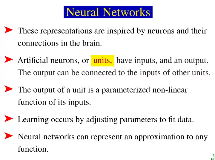
Neural Networks ➤ These representations are inspired by neurons and their connections in the brain. ➤ Artificial neurons, or units, have inputs, and an output. The output can be connected to the inputs of other units. ➤ The output of a unit is a parameterized non-linear function of its inputs. ➤ Learning occurs by adjusting parameters to fit data. ➤ Neural networks can represent an approximation to any function. ☞ ☞
Why Neural Networks? ➤ As part of neuroscience, in order to understand real neural systems, researchers are simulating the neural systems of simple animals such as worms. ➤ It seems reasonable to try to build the functionality of the brain via the mechanism of the brain (suitably abstracted). ➤ The brain inspires new ways to think about computation. ➤ Neural networks provide a different measure of simplicity as a learning bias. ☞ ☞ ☞
Feed-forward neural networks ➤ Feed-forward neural networks are the most common models. ➤ These are directed acyclic graphs: output hidden inputs units ☞ units ☞ ☞
The Units A unit with k inputs is like the parameterized logic program: prop ( Obj , output , V ) ← prop ( Obj , in 1 , I 1 ) ∧ prop ( Obj , in 2 , I 2 ) ∧ · · · prop ( Obj , in k , I k ) ∧ V is f ( w 0 + w 1 × I 1 + w 2 × I 2 + · · · + w k × I k ). ➤ I j are real-valued inputs. ➤ w j are adjustable real parameters. ➤ f is an activation function. ☞ ☞ ☞
Activation function A typical activation function is the sigmoid function: 1 0.9 1 0.8 0.7 1 + e x 0.6 0.5 0.4 0.3 0.2 0.1 0 -10 -5 0 5 10 1 f ′ ( x ) = f ( x )( 1 − f ( x )) f ( x ) = 1 + e − x ☞ ☞ ☞
Neural Network for the news example inputs hidden output units units known new reads short home ☞ ☞ ☞
Axiomatizing the Network ➤ The values of the attributes are real numbers. ➤ Thirteen parameters w 0 , . . . , w 12 are real numbers. ➤ The attributes h 1 and h 2 correspond to the values of hidden units. ➤ There are 13 real numbers to be learned. The hypothesis space is thus a 13-dimensional real space. ➤ Each point in this 13-dimensional space corresponds to a particular logic program that predicts a value for reads given known , new , short , and home . ☞ ☞ ☞
predicted _ prop ( Obj , reads , V ) ← prop ( Obj , h 1 , I 1 ) ∧ prop ( Obj , h 2 , I 2 ) ∧ V is f ( w 0 + w 1 × I 1 + w 2 × I 2 ). prop ( Obj , h 1 , V ) ← prop ( Obj , known , I 1 ) ∧ prop ( Obj , new , I 2 ) ∧ prop ( Obj , short , I 3 ) ∧ prop ( Obj , home , I 4 ) ∧ V is f ( w 3 + w 4 × I 1 + w 5 × I 2 + w 6 × I 3 + w 7 × I 4 ). prop ( Obj , h 2 , V ) ← prop ( Obj , known , I 1 ) ∧ prop ( Obj , new , I 2 ) ∧ prop ( Obj , short , I 3 ) ∧ prop ( Obj , home , I 4 ) ∧ V is f ( w 8 + w 9 × I 1 + w 10 × I 2 + w 11 × I 3 + w 12 × I 4 ). ☞ ☞ ☞
Prediction Error ➤ For particular values for the parameters w = w 0 , . . . w m and a set E of examples, the sum-of-squares error is � ( p w e − o e ) 2 , Error E ( w ) = e ∈ E ➣ p w e is the predicted output by a neural network with parameter values given by w for example e ➣ o e is the observed output for example e . ➤ The aim of neural network learning is, given a set of examples, to find parameter settings that minimize the error. ☞ ☞ ☞
Neural Network Learning ➤ Aim of neural network learning: given a set of examples, find parameter settings that minimize the error. ➤ Back-propagation learning is gradient descent search through the parameter space to minimize the sum-of-squares error. ☞ ☞ ☞
Backpropagation Learning ➤ Inputs: ➣ A network, including all units and their connections ➣ Stopping Criteria ➣ Learning Rate (constant of proportionality of gradient descent search) ➣ Initial values for the parameters ➣ A set of classified training data ➤ Output: Updated values for the parameters ☞ ☞ ☞
Backpropagation Learning Algorithm ➤ Repeat ➣ evaluate the network on each example given the current parameter settings ➣ determine the derivative of the error for each parameter ➣ change each parameter in proportion to its derivative ➤ until the stopping criteria is met ☞ ☞ ☞
Gradient Descent for Neural Net Learning ➤ At each iteration, update parameter w i � � w i − η∂ error ( w i ) w i ← ∂ w i η is the learning rate ➤ You can compute partial derivative: ➣ numerically: for small � error ( w i + �) − error ( w i ) � ➣ analytically: f ′ ( x ) = f ( x )( 1 − f ( x )) + chain rule ☞ ☞ ☞
Simulation of Neural Net Learning Para- iteration 0 iteration 1 iteration 80 meter Value Deriv Value Value w 0 0 . 2 0 . 768 − 0 . 18 − 2 . 98 w 1 0 . 12 0 . 373 − 0 . 07 6 . 88 0 . 112 0 . 425 − 0 . 10 − 2 . 10 w 2 w 3 0 . 22 0 . 0262 0 . 21 − 5 . 25 w 4 0 . 23 0 . 0179 0 . 22 1 . 98 Error: 4 . 6121 4 . 6128 0 . 178 ☞ ☞ ☞
What Can a Neural Network Represent? w 2 I 2 w 0 w 1 w 2 Logic -15 10 10 and w 1 -5 10 10 or I 1 w 0 5 -10 -10 nor Output is f ( w 0 + w 1 × I 1 + w 2 × I 2 ) . A single unit can’t represent xor . ☞ ☞ ☞
Bias in neural networks and decision trees ➤ It’s easy for a neural network to represent “at least two of I 1 , . . . , I k are true”: w 0 w 1 w k · · · -15 10 10 · · · This concept forms a large decision tree. ➤ Consider representing a conditional: “If c then a else b ”: ➣ Simple in a decision tree. ➣ Needs a complicated neural network to represent ( c ∧ a ) ∨ ( ¬ c ∧ b ) . ☞ ☞ ☞
Neural Networks and Logic ➤ Meaning is attached to the input and output units. ➤ There is no a priori meaning associated with the hidden units. ➤ What the hidden units actually represent is something that’s learned. ☞ ☞
Recommend
More recommend
Explore More Topics
Stay informed with curated content and fresh updates.
