Neural Networks (Perceptrons) A mathematical perspective Textbook - PowerPoint PPT Presentation
Neural Networks (Perceptrons) A mathematical perspective Textbook reference: Sections 11.1-11.2 Additional Reference: Nillson, N. Artificial Intelligence: A New Synthesis , San Francisco: Morgan Kaufmann, 1998. (Chapter 2, Chapter 3 (3.1 -
Neural Networks (Perceptrons) A mathematical perspective Textbook reference: Sections 11.1-11.2 Additional Reference: Nillson, N. Artificial Intelligence: A New Synthesis , San Francisco: Morgan Kaufmann, 1998. (Chapter 2, Chapter 3 (3.1 - 3.2)) . – p.1/30
Neural networks (NNs) Nilsson (1998) refers to them as "stimulus response agents". Agents behave based on motor responses stimulated by immediate sensory inputs. They "learn" these motor responses through exposure to a set of samples of inputs paired with the action that would be appropriate for each input. We are focusing on "engineering" such networks rather than studying biological neurons. . – p.2/30
An artificial neuron x1 n Σ x2 w1 xi wi w2 Output, f i=1 Σ wi xi wn Threshold, Θ xn n Σ = 1 if Θ f xi wi i=1 = 0 otherwise Remember that a single neuron is capable of two actions corresponding to the two possible outputs of the neuron. . – p.3/30
� ✁ ✂ The learning problem We are given a set, T, of n-dimensional vectors, X , with components , = 1 , . . . , n. These vectors are feature vectors computed by the perceptual processing component of a reactive agent. The values can be real or Boolean. For each X in T, we also know the appropriate action, a. These associated actions are sometimes called the labels or the classes of the vectors. . – p.4/30
✄ � � ✂ ✁ The learning problem (cont’d) The set T and the associated labels are called the training set . The machine learning problem is to find a function, say, , that responds "acceptably" to the members of the training set. Remember that this type of learning is supervised . We would like the action computed by to agree with the label for as many vectors in T as possible. . – p.5/30
� Training a single neuron Equation of hyperplane − Θ = 0 X . W − Θ > 0 X . W W Unit vector normal on this side to hyperplane |W| − Θ < 0 X . W Origin on this side adjusting the threshold changes the position of the hyperplane boundary with respect to the origin adjusting the weights changes the orientation of the hyperplane . – p.6/30
� Augmented vectors The procedure is simplified if we use a threshold of 0 rather than an arbitrary threshold. This can be achieved by using (n+1)-dimensional "augmented" vectors. The (n+1)-th component of the augmented input vector always has value 1; the weight of the (n+1)-th component is set to the negative of the desired threshold value, . . – p.7/30
� � � ✁ Augmented vectors (cont’d) So rather than checking X . W against , we check X . W - against 0. Using augmented vectors, the output of the neuron is 1 when X . W , and 0 otherwise. . – p.8/30
✞ � � ✁ ✂ ✁ ✁ � ✠ ✄ ✁ ✟ ✁ ✁ ✞ ✁ ✝ ✆ ✁ � Gradient Descent Method Define an error function that can be minimized by adjusting weight values. A commonly used error function is squared error: ✂☎✄ where is the actual response for input , and is the desired response. For fixed T, we see that the error depends on the weight values through . . – p.9/30
� � � Gradient Descent Method (cont’d) A gradient descent process is useful to find the minimum of : calculate the gradient of in weight space and move the weight vector along the negative gradient (downhill). Note that, as defined, depends on all the input vectors in S. Use one vector at a time incrementally rather than all at once. Note that, the incremental process is an approximation of the “batch” process. Nevertheless, it works. . – p.10/30
Gradient Descent Method (cont’d) The following is a hypothetical error surface in two dimensions. Constant c dictates the size of the learning step. E W old c W new local minimum error surface W . – p.11/30
� The procedure Take one member of T. Adjust the weights if needed. Repeat (a predefined number of times or until is sufficiently small.) . – p.12/30
✂ � ✄ ✁ � ✁ ✁ ☎ ✝ � � ✁ ✝ ✁ � ✂ ✁ ☎ ✁ ✝ � ✁ ✂ � ✁ ✂ ☛ ✆ � ✡ ✞ ✁ � ✁ ✞ � ✟ � ✄ ✠ � ✂ � � ✁ � How to adjust the weights The squared error for a single output vector, , evoking an output of , when the desired output is is: The gradient of with respect to the weights is . ☎✠✟ ✆✞✝ . – p.13/30
✂ ✁ ✞ ✁ ✄ ✟ ✁ ✁ ✂ � � ✁ � ✂ ✂ ✁ ✟ ✄ ✂ ✁ ✟ ✞ ✁ ✄ ✟ ✁ ✂ ✁ � ✁ ✁ ✁ ✁ ✂ � ✁ � ✄ � ✂ � ✁ ✁ ✁ ✂ ✁ ✁ ✁ ✂ ✂ ✁ � � ✁ ✂ ✁ ✁ ✁ ✁ ✂ � ✁ ✂ ✁ ✁ ✂ ✁ ✁ ✁ ✁ ✂ ✁ � How to adjust the weights (cont’d) Since dependence on W is entirely through the dot product, s = X . W, we can use the chain rule to write Because Note that . Thus . – p.14/30
✁ � ✁ � ✂ ✁ ✁ � � How to adjust the weights (cont’d) The remaining problem is to compute . The perceptron output, , is not continuously differentiable with respect to because of the presence of the threshold function. Most small changes in the dot product do not change at all, and when does change, it changes abruptly from 1 to 0 or vice versa. We will look at two methods to compute the differential. . – p.15/30
� ✁ ✁ Computing the differential Ignore the threshold function and let . ( The Widrow-Hoff Procedure ). Replace the threshold function with another nonlinear function that is differentiable ( The Generalized Delta Procedure ). . – p.16/30
✠ ✂ ✁ ✄ ✁ ✄ ✁ � ✁ ✞ ✁ ✁ � ✟ ✁ ✁ � ✟ ✁ ✁ ✞ ✂ ✄ � ✟ � ✁ ✁ � ✁ ✁ ✁ ✞ ✟ � ✄ ✠ ✂ The Widrow-Hoff Procedure Suppose we attempt to adjust the weights so that every training vector labeled with a 1 produces a dot product of exactly 1, and every vector labeled with a 0 produces a dot product of exactly -1. In that case, with , , and, . Now, the gradient is . – p.17/30
� ✁ ✞ ✟ � ✄ ✂ The Widrow-Hoff Proc. (cont’d) Moving the weight vector along the negative gradient, and incorporating the factor 2, into a learning rate parameter , c , the new value of the weight vector is given by ✁✄✂ All we need to do now is to plug in this formula in the "adjust the weights" step of the training procedure. . – p.18/30
✞ ✁ ✟ ✄ � ✟ ✞ ✁ � ✄ ✄ � ✟ ✞ ✁ ✂ ✄ � ✟ ✞ ✁ ✂ ✁ � The Widrow-Hoff Proc. (cont’d) We have, . Whenever is positive, we add a fraction of the input vector into the weight vector. This addition makes the dot product larger, and smaller. Similarly, when is negative, we subtract a fraction of the input vector from the weight vector. . – p.19/30
� ✁ ✁ � The Widrow-Hoff Proc. (cont’d) This procedure is also known as the Delta rule . After finding a set of weights that minimize the squared error (using ), we are free to revert to the threshold function for . . – p.20/30
� ✂ � ✁ ✝ � ✁ ✁ ✄ ✁ � ✂ ✁ ✄ ✄ The generalized Delta procedure Another way of dealing with the nondifferentiable threshold function: replace the threshold function by an S-shaped differentiable function called a sigmoid . Usually, the sigmoid function used is: where is the input and is the ✁ ✁� output. . – p.21/30
A Sigmoid Function 1.0 0.8 0.6 0.4 0.2 −6 −4 −2 2 4 6 It is possible to get sigmoid functions of different “flatness” by adjusting the exponent. . – p.22/30
� � ✄ ✂ ✁ ✁ ✟ ✄ ✁ ✞ ✟ � ✄ � ✁ ✟ ✂ � ✄ ✂ ✂ � � ✟ ✁ ✞ ✟ � ✄ � ✁ ✂ � ✁ ✁ � ✂ ✁ ✁ ✁ � ✁ � ✟ � ✄ ✂ � ✁ ✂ ✁ ✁ ✟ ✄ ✁ ✞ ✟ � ✄ ✁ � ✂ ✁ ✁ The generalized Delta procedure (cont’d) With the sigmoid function, Substitute into The new weight change rule is: ✁✄✂ . – p.23/30
� ✞ ✁ Comparison Compare Widrow-Hoff and Generalized Delta: the desired output, , Widrow-Hoff: either 1 or -1, Generalized Delta: either 1 or 0. the actual output, , Widrow-Hoff: equals , the dot product, Generalized Delta: the sigmoid function. The sigmoid can be thought of implementing a “fuzzy” hyperplane. . – p.24/30
✄ � � ✟ � � ✄ � � ✟ � ✁ � � � ✁ ✄ � ✄ � ✁ � ✟ � ✄ � � � ✟ � ✁ � ✟ ✁ Fuzzy hyperplane In generalized Delta, there is the added term due to the presence of the sigmoid function. When = 0, is also 0. When = 1, is 0. When = 1/2, reaches its maximum value (1/4). Weight changes are made where changes have much effect on . For an input vector far away from the fuzzy hyperplane, has value closer to 0, and the generalized Delta rule makes little or no change to the weight values regardless of the desired output. . – p.25/30
Recommend
More recommend
Explore More Topics
Stay informed with curated content and fresh updates.
![CS485/685 Lecture 7: Jan 24, 2012 Perceptrons, Neural Networks [B]: Sections 4.1.7, 5.1 CS485/685](https://c.sambuz.com/732798/cs485-685-lecture-7-jan-24-2012-s.webp)
![CS480/680 Lecture 9: June 5, 2019 Perceptrons, Neural Networks [D] Chapt. 4, [HTF] Chapt. 11,](https://c.sambuz.com/690997/cs480-680-lecture-9-june-5-2019-s.webp)

![Declaring Array Variables Chapter 6 Arrays datatype[] arrayRefVar; Preferred! Example:](https://c.sambuz.com/1036956/declaring-array-variables-chapter-6-arrays-s.webp)
