Neural Networks Linear regression (again) Radial basis function - - PowerPoint PPT Presentation

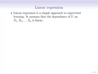
Neural Networks

• Linear regression (again)
• Radial basis function networks
• Self-organizing maps
• Recurrent networks

Partially based on slides by John A. Bullinaria and J. Kok

Linear Regression

1 2 3 4 5 1 2 3 4 5 6 7

Linear Regression

Search for such that is small for all i Add to find intercept

Linear Regression

Example:

1 2 3 4 5 1 2 3 4 5 6 7

Linear Regression

Error function: Compute global minimum by means of derivative:

Linear Regression

Compute global minimum by means of derivative:

Linear Regression

Compute global minimum by means of derivative:

Linear Regression

Online learning; given one example, the error is: Taking the derivative with respect to one weight: Update weight:

Radial Basis Function Networks

Localized activation function Weighted sum or average output

Ri( x)=e(−

∥x−ui∥

2

2σi

2 )

Ri( x)=1/(1+e

−

∥x−u i∥

2

σ i

2 )

d( x)=∑

i=1 H

ci Ri(x )

d( x)=∑i=1

H

ci Ri( x)

∑i=1

H

Ri( x )

RBF is not a multi-layered perceptron

Weighted sum Weighted average

Hidden layer Hidden layer Localized activation functions in the hidden layer

RBFN Example

RBFN Example

RBFN Learning

Three types of parameters:

centers of the radial basis functions width of the radial basis functions weights for each radial basis function

“Obvious” algorithm: backpropagation?

RBFN Hybrid Learning

Step 1: Fix the RBF centers and widths Step 2: Learn the linear weights

RBFN Hybrid Learning

Step 1: Fixed selection

RBFN Hybrid Learning

Step 1: Clustering

RBFN Hybrid Learning

Step 2: linear regression!

• 1. Calculate for each pattern its (normalized) RBF

value, for each of the neurons

• 2. Create a table:
• 3. Linear regression

Output Neuron 1 Output Neuron 2 ... Output Neuron n Desired Output ... ... ... ... ...

RBFN vs MLP

The hidden layer of a RBFN does not compute a weighted sum, but a distance to a

center

The layers of a RBFN are usually trained one layer at a time RBFNs consitute a set of local models, MPLs represent a global model A RBFN will predict 0 when it doesn't know anything The number of neurons in a RBFN for accurate prediction can be high Removing one neuron can have a large influence

RBFN vs Sugeno Systems?

Self-Organising Maps (Kohonen Networks)

Unsupervised setting These networks can be used to

cluster a space of patterns learn nodes in hidden layer of a RBFN map a high dimensional space to a lower dimensional

• ne

solving traveling salesman problems heuristically

Kohonen Networks

Example: network in a grid structure

Kohonen Networks

1 2 3 4 5 ... 1 2 3 ... Mapping such that points close in input are close in output

Kohonen Networks

Solving a traveling salesman problem using a network

in a circular structure: cities close on a map should be close on the tour

(Elastic net)

Kohonen Networks: Algorithm

Step 1: initialize weights for each node at random Step 2: sample a training pattern Step 3: compute which node is closest to the sample Step 4: adapt the weights of this node such that this node is even closer

to the pattern next time

Step 5: adapt the weight of closeby nodes (in the grid, on the line, …)

such that also these other nodes are close

Go to step 2

Kohonen Networks: Algorithm

Step 3: distance calculation for node i Step 4: adapt weights for node i (update rule)

Kohonen Networks: Algorithm

Step 5: adapt weights of nodes closeby

Step 5a: calculate distance d(i,i*) between two nodes in the grid / on the line Step 5b: reweigh the distance (closeby = high weight) Step 5c: update weight nearby

Kohonen Networks: Illustration

Kohonen Networks: Defects

Avoiding “knots”:

higher σ higher learning rate

in early iterations

Kohonen Networks: Examples

5000 uniform samples from 2D space 80000 samples 50000 samples 70000 samples

Kohonen Networks: Examples

Uniform Not uniform

Kohonen Networks: Examples

Kohonen Networks

How to use for clustering? How to use to build RBF networks?

Recurrent Networks

The output of any neuron can be the input of any

• ther

Hopfield (Recurrent) Network

Input = activation: {-1,1} Activation function:

Hopfield Network: Input Processing

Given an input Asynchronously: (Common)

Step 1: sample an arbitrary unit Step 2: update its activation Step 3: if activation does not change, stop, otherwise repeat

Synchronously:

Step 1: save all current activations (time t) Step 2: recompute activation for all units a time t+1 using

activations at time t

Step 3: if activation does not change, stop, otherwise repeat

Hopfield Network: Associative Memory

Patterns “stored” in

the network:

Retrieval task: for given input, find the input that is

closest:

Activation over time, given input

Hopfield Network: Learning

Activation:

Hopfield Network: Learning

Definition A network is stable for one pattern if:

where is a pattern

If we pick the weights as follows, the network will be

stable for pattern : (N is number of units)

Hopfield Network: Learning

Proof for stability:

Hopfield Network: Learning

Learning multiple patterns: “Hebb rule” Ensures that with a high probability approximately

0.139N arbitrary patterns can be stored (no proof given)

Simple learning algorithm: assign all weights once!

Hopfield Network: Learning

Intuition

with high probability for 0.139N patterns

<0.5

Hopfield Network: Energy Function

We define the energy of network activation as: We will show that energy always goes down when

updating activations

Assume we recalculate unit i:

… and that its activation changes

Hopfield Network: Energy Function

Calculate change in energy

Hopfield Network: Energy Function

Choose as energy function

this function has local minima at each of the patterns

Rewrite:

Note: if , this is 1, sum total is N (maximal)

Next week

More on recurrent networks Deep belief networks Slowly moving to variations of evolutionary

algorithms