Neural Networks 2/2 Many slides attributable to: Prof. Mike Hughes - PowerPoint PPT Presentation
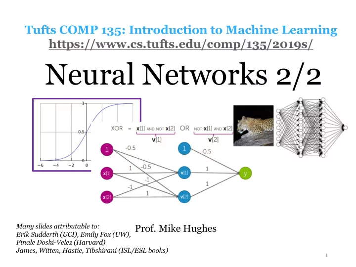
Tufts COMP 135: Introduction to Machine Learning https://www.cs.tufts.edu/comp/135/2019s/ Neural Networks 2/2 Many slides attributable to: Prof. Mike Hughes Erik Sudderth (UCI), Emily Fox (UW), Finale Doshi-Velez (Harvard) James, Witten,
Tufts COMP 135: Introduction to Machine Learning https://www.cs.tufts.edu/comp/135/2019s/ Neural Networks 2/2 Many slides attributable to: Prof. Mike Hughes Erik Sudderth (UCI), Emily Fox (UW), Finale Doshi-Velez (Harvard) James, Witten, Hastie, Tibshirani (ISL/ESL books) 1
Logistics • Project 1: Keep going! • Recitation tonight Monday • Hands-on intro to neural nets • With automatic differentiation • HW4 out on Wed, due in TWO WEEKS Mike Hughes - Tufts COMP 135 - Spring 2019 2
Objectives Today : Neural Networks Unit 2/2 • Review: learning feature representations • Feed-forward neural nets (MLPs) • Activation functions • Loss functions for multi-class classification • Training via gradient descent • Back-propagation = gradient descent + chain rule • Automatic differentiation Mike Hughes - Tufts COMP 135 - Spring 2019 3
What will we learn? Evaluation Supervised Training Learning Data, Label Pairs Performance { x n , y n } N measure Task n =1 Unsupervised Learning data label x y Reinforcement Learning Prediction Mike Hughes - Tufts COMP 135 - Spring 2019 4
Task: Binary Classification y is a binary variable Supervised (red or blue) Learning binary classification x 2 Unsupervised Learning Reinforcement Learning x 1 Mike Hughes - Tufts COMP 135 - Spring 2019 5
Feature Transform Pipeline Data, Label Pairs { x n , y n } N n =1 Feature, Label Pairs Performance Task { φ ( x n ) , y n } N measure n =1 label data φ ( x ) y x Mike Hughes - Tufts COMP 135 - Spring 2019 6
Logistic Regr. Network Diagram 0 or 1 Credit: Emily Fox (UW) https://courses.cs.washington.edu/courses/cse41 6/18sp/slides/ Mike Hughes - Tufts COMP 135 - Spring 2019 7
Multi-class Classification How to do this? Mike Hughes - Tufts COMP 135 - Spring 2019 8
Binary Prediction Goal: Predict label (0 or 1) given features x x i , [ x i 1 , x i 2 , . . . x if . . . x iF ] • Input: “features” Entries can be real-valued, or “covariates” other numeric types (e.g. integer, binary) “attributes” y i ∈ { 0 , 1 } • Output: Binary label (0 or 1) “responses” or “labels” >>> yhat_N = model. predict (x_NF) >>> yhat_N[:5] [0, 0, 1, 0, 1] Mike Hughes - Tufts COMP 135 - Spring 2019 9
Binary Proba. Prediction Goal: Predict probability of label given features x i , [ x i 1 , x i 2 , . . . x if . . . x iF ] • Input: “features” Entries can be real-valued, or “covariates” other numeric types (e.g. integer, binary) “attributes” p i , p ( Y i = 1 | x i ) • Output: ˆ Value between 0 and 1 e.g. 0.001, 0.513, 0.987 “probability” >>> yproba_N2 = model. predict_proba (x_NF) >>> yproba1_N = model. predict_proba (x_NF) [:,1] >>> yproba1_N[:5] [0.143, 0.432, 0.523, 0.003, 0.994] Mike Hughes - Tufts COMP 135 - Spring 2019 10
Multi-class Prediction Goal: Predict one of C classes given features x x i , [ x i 1 , x i 2 , . . . x if . . . x iF ] • Input: “features” Entries can be real-valued, or “covariates” other numeric types (e.g. integer, binary) “attributes” • Output: y i ∈ { 0 , 1 , 2 , . . . C − 1 } Integer label (0 or 1 or … or C-1 ) “responses” or “labels” >>> yhat_N = model. predict (x_NF) >>> yhat_N[:6] [0, 3, 1, 0, 0, 2] Mike Hughes - Tufts COMP 135 - Spring 2019 11
Multi-class Proba. Prediction Goal: Predict probability of label given features Input: x i , [ x i 1 , x i 2 , . . . x if . . . x iF ] “features” Entries can be real-valued, or other “covariates” numeric types (e.g. integer, binary) “attributes” Output: p i , [ p ( Y i = 0 | x i ) ˆ p ( Y i = 1 | x i ) . . . p ( Y i = C − 1 | x i )] “probability” Vector of C non-negative values, sums to one >>> yproba_NC = model. predict_proba (x_NF) >>> yproba_c_N = model. predict_proba (x_NF) [:,c] >>> np.sum(yproba_NC, axis=1) [1.0, 1.0, 1.0, 1.0] Mike Hughes - Tufts COMP 135 - Spring 2019 12
From Real Value to Probability probability 1 sigmoid( z ) = 1 + e − z Mike Hughes - Tufts COMP 135 - Spring 2019 13
From Vector of Reals to Vector of Probabilities z i = [ z i 1 z i 2 . . . z ic . . . z iC ] " # e z i 1 e z i 2 e z iC p i = ˆ c =1 e z ic . . . . . . P C P C P C c =1 e z ic c =1 e z ic called the “softmax” function Mike Hughes - Tufts COMP 135 - Spring 2019 14
Representing multi-class labels y n ∈ { 0 , 1 , 2 , . . . C − 1 } ∈ { − } Encode as length-C one hot binary vector y n = [¯ ¯ y n 1 ¯ y n 2 . . . ¯ y nc . . . ¯ y nC ] Examples (assume C=4 labels) class 0: [1 0 0 0] class 1: [0 1 0 0] class 2: [0 0 1 0] class 3: [0 0 0 1] Mike Hughes - Tufts COMP 135 - Spring 2019 15
“Neuron” for Binary Prediction Probability of class 1 Logistic sigmoid Linear function activation with weights w function Credit: Emily Fox (UW) Mike Hughes - Tufts COMP 135 - Spring 2019 16
Neurons for Multi-class Prediction • Can you draw it? Mike Hughes - Tufts COMP 135 - Spring 2019 17
Recall: Binary log loss ( 1 if y 6 = ˆ y error( y, ˆ y ) = 0 if y = ˆ y log loss( y, ˆ p ) = − y log ˆ p − (1 − y ) log(1 − ˆ p ) Plot assumes: - True label is 1 - Threshold is 0.5 - Log base 2 Mike Hughes - Tufts COMP 135 - Spring 2019 18
Multi-class log loss Input: two vectors of length C Output: scalar value (strictly non-negative) C X log loss(¯ y n , ˆ p n ) = − y nc log ˆ ¯ p nc c =1 Justifications carry over from the binary case: - Interpret as upper bound on the error rate - Interpret as cross entropy of multi-class discrete random variable - Interpret as log likelihood of multi-class discrete random variable Mike Hughes - Tufts COMP 135 - Spring 2019 19
MLP: Multi-Layer Perceptron 1 or more hidden layers followed by 1 output layer Mike Hughes - Tufts COMP 135 - Spring 2019 20
Linear decision boundaries cannot solve XOR X_1 X_2 y 0 0 0 0 1 1 1 0 1 1 1 0 Mike Hughes - Tufts COMP 135 - Spring 2019 21
Diagram of an MLP f 1 ( x, w 1 ) f 2 ( · , w 2 ) f 3 ( · , w 3 ) Input data Output x Mike Hughes - Tufts COMP 135 - Spring 2019 22
Each Layer Extracts “Higher Level” Features Mike Hughes - Tufts COMP 135 - Spring 2019 23
MLPs with 1 hidden layer can approximate any functions with enough hidden units! Mike Hughes - Tufts COMP 135 - Spring 2019 24
Which Activation Function? Linear function Non-linear activation with weights w function Credit: Emily Fox (UW) Mike Hughes - Tufts COMP 135 - Spring 2019 25
Activation Functions Mike Hughes - Tufts COMP 135 - Spring 2019 26
How to train Neural Nets? Just like logistic regression Set up a loss function Apply Gradient Descent! Mike Hughes - Tufts COMP 135 - Spring 2019 27
Review: LR notation • Feature vector with first entry constant • Weight vector (first entry is the “bias”) w = [ w 0 w 1 w 2 . . . w F ] • “Score” value z (real number, -inf to +inf) Mike Hughes - Tufts COMP 135 - Spring 2019 28
Review: Gradient of LR Log likelihood J ( z n ( w )) = y n z n − log(1 + e z n ) d d d Gradient w.r.t. weight on feature f − d d d J ( z n ( w )) = J ( z n ) · z ( w ) dw f dz n dw f chain rule! Mike Hughes - Tufts COMP 135 - Spring 2019 29
MLP : Composable Functions f 1 ( x, w 1 ) f 2 ( · , w 2 ) f 3 ( · , w 3 ) Input data x Mike Hughes - Tufts COMP 135 - Spring 2019 30
Output as function of x f 3 ( f 2 ( f 1 ( x, w 1 ) , w 2 ) , w 3 ) f 1 ( x, w 1 ) f 2 ( · , w 2 ) f 3 ( · , w 3 ) Input data x Mike Hughes - Tufts COMP 135 - Spring 2019 31
Minimizing loss for composable functions N X min loss( y n , f 3 ( f 2 ( f 1 ( x n , w 1 ) , w 2 ) , w 3 ) w 1 ,w 2 ,w 3 n =1 Loss can be: • Squared error for regression problems • Log loss for multi-way classification problems • … many others possible! Mike Hughes - Tufts COMP 135 - Spring 2019 32
Compute loss via Forward Propagation w (1) b (1) w (2) b (2) Mike Hughes - Tufts COMP 135 - Spring 2019 33
Compute loss via Forward Propagation w (1) b (1) w (2) b (2) Step 2: Mike Hughes - Tufts COMP 135 - Spring 2019 34
Compute loss via Forward Propagation w (1) b (1) w (2) b (2) Step 2: Step 3: Mike Hughes - Tufts COMP 135 - Spring 2019 35
Compute gradient via Back Propagation w (1) b (1) w (2) b (2) w (1) b (1) w (2) b (2) Visual Demo: https://google-developers.appspot.com/machine- learning/crash-course/backprop-scroll/ Mike Hughes - Tufts COMP 135 - Spring 2019 36
Network view of Backprop Mike Hughes - Tufts COMP 135 - Spring 2019 37
Is Symbolic Differentiation the only way to compute derivatives? Credit: Justin Domke (UMass) https://people.cs.umass.edu/~domk e/courses/sml/09autodiff_nnets.pdf Mike Hughes - Tufts COMP 135 - Spring 2019 38
Another view: Credit: Justin Domke (UMass) https://people.cs.umass.edu/~domk e/courses/sml/09autodiff_nnets.pdf Computation graph Mike Hughes - Tufts COMP 135 - Spring 2019 39
Credit: Justin Domke (UMass) Forward https://people.cs.umass.edu/~domk e/courses/sml/09autodiff_nnets.pdf Propagation Mike Hughes - Tufts COMP 135 - Spring 2019 40
Recommend
More recommend
Explore More Topics
Stay informed with curated content and fresh updates.
