Near-optimal Algorithms for Online Linear Programming Zizhuo Wang - PowerPoint PPT Presentation
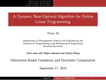
Near-optimal Algorithms for Online Linear Programming Zizhuo Wang Department of Industrial and Systems Engineering University of Minnesota Joint work with Shipra Agrawal and Yinyu Ye July 7th, 2014 Zizhuo Wang Online Linear Programs, TOLA
Near-optimal Algorithms for Online Linear Programming Zizhuo Wang Department of Industrial and Systems Engineering University of Minnesota Joint work with Shipra Agrawal and Yinyu Ye July 7th, 2014 Zizhuo Wang Online Linear Programs, TOLA
Introduction Zizhuo Wang Online Linear Programs, TOLA
Introduction In traditional optimization problems, the input data is given (either in deterministic form or stochastic form). Zizhuo Wang Online Linear Programs, TOLA
Introduction In traditional optimization problems, the input data is given (either in deterministic form or stochastic form). For example, in a linear program π T x maximize x subject to A x = b x ≥ 0 , one solves the decision variables all at once. Zizhuo Wang Online Linear Programs, TOLA
Introduction In traditional optimization problems, the input data is given (either in deterministic form or stochastic form). For example, in a linear program π T x maximize x subject to A x = b x ≥ 0 , one solves the decision variables all at once. However, in many practical problems, the input information is not available at the start, but reveals sequentially. Decisions have to be made in an online fashion. Zizhuo Wang Online Linear Programs, TOLA
Introduction In traditional optimization problems, the input data is given (either in deterministic form or stochastic form). For example, in a linear program π T x maximize x subject to A x = b x ≥ 0 , one solves the decision variables all at once. However, in many practical problems, the input information is not available at the start, but reveals sequentially. Decisions have to be made in an online fashion. ◮ Online linear programming problems Zizhuo Wang Online Linear Programs, TOLA
Introduction Zizhuo Wang Online Linear Programs, TOLA
Introduction In this talk, we consider linear programs of the following format: � n maximize x t =1 π t x t � n subject to t =1 a it x t ≤ B i , ∀ i = 1 , ..., m 0 ≤ x t ≤ 1 , ∀ t = 1 , ..., n Zizhuo Wang Online Linear Programs, TOLA
Introduction In this talk, we consider linear programs of the following format: � n maximize x t =1 π t x t � n subject to t =1 a it x t ≤ B i , ∀ i = 1 , ..., m 0 ≤ x t ≤ 1 , ∀ t = 1 , ..., n In the online version of the problem: we only know B i ’s at the start. Zizhuo Wang Online Linear Programs, TOLA
Introduction In this talk, we consider linear programs of the following format: � n maximize x t =1 π t x t � n subject to t =1 a it x t ≤ B i , ∀ i = 1 , ..., m 0 ≤ x t ≤ 1 , ∀ t = 1 , ..., n In the online version of the problem: we only know B i ’s at the start. ◮ The constraint matrix is revealed column by column sequentially along with the corresponding objective coefficient. Zizhuo Wang Online Linear Programs, TOLA
Introduction In this talk, we consider linear programs of the following format: � n maximize x t =1 π t x t � n subject to t =1 a it x t ≤ B i , ∀ i = 1 , ..., m 0 ≤ x t ≤ 1 , ∀ t = 1 , ..., n In the online version of the problem: we only know B i ’s at the start. ◮ The constraint matrix is revealed column by column sequentially along with the corresponding objective coefficient. ◮ An irrevocable decision must be made as soon as a column arrives without observing or knowing the future data. Zizhuo Wang Online Linear Programs, TOLA
Applications Zizhuo Wang Online Linear Programs, TOLA
Applications � n maximize x t =1 π t x t � n subject to t =1 a it x t ≤ B i , ∀ i = 1 , ..., m 0 ≤ x t ≤ 1 , ∀ t = 1 , ..., n Zizhuo Wang Online Linear Programs, TOLA
Applications � n maximize x t =1 π t x t � n subject to t =1 a it x t ≤ B i , ∀ i = 1 , ..., m 0 ≤ x t ≤ 1 , ∀ t = 1 , ..., n This model is frequently used in resource allocation problems. Zizhuo Wang Online Linear Programs, TOLA
Applications � n maximize x t =1 π t x t � n subject to t =1 a it x t ≤ B i , ∀ i = 1 , ..., m 0 ≤ x t ≤ 1 , ∀ t = 1 , ..., n This model is frequently used in resource allocation problems. ◮ { a it } m i =1 are the request of a bundle of goods by t th customer Zizhuo Wang Online Linear Programs, TOLA
Applications � n maximize x t =1 π t x t � n subject to t =1 a it x t ≤ B i , ∀ i = 1 , ..., m 0 ≤ x t ≤ 1 , ∀ t = 1 , ..., n This model is frequently used in resource allocation problems. ◮ { a it } m i =1 are the request of a bundle of goods by t th customer ◮ B i is the inventory for the i th good. Zizhuo Wang Online Linear Programs, TOLA
Applications � n maximize x t =1 π t x t � n subject to t =1 a it x t ≤ B i , ∀ i = 1 , ..., m 0 ≤ x t ≤ 1 , ∀ t = 1 , ..., n This model is frequently used in resource allocation problems. ◮ { a it } m i =1 are the request of a bundle of goods by t th customer ◮ B i is the inventory for the i th good. ◮ π t is the price that the t th customer is willing to pay. Zizhuo Wang Online Linear Programs, TOLA
Applications � n maximize x t =1 π t x t � n subject to t =1 a it x t ≤ B i , ∀ i = 1 , ..., m 0 ≤ x t ≤ 1 , ∀ t = 1 , ..., n This model is frequently used in resource allocation problems. ◮ { a it } m i =1 are the request of a bundle of goods by t th customer ◮ B i is the inventory for the i th good. ◮ π t is the price that the t th customer is willing to pay. ◮ x t is the decision whether to accept or reject the t th customer Zizhuo Wang Online Linear Programs, TOLA
Applications � n maximize x t =1 π t x t � n subject to t =1 a it x t ≤ B i , ∀ i = 1 , ..., m 0 ≤ x t ≤ 1 , ∀ t = 1 , ..., n This model is frequently used in resource allocation problems. ◮ { a it } m i =1 are the request of a bundle of goods by t th customer ◮ B i is the inventory for the i th good. ◮ π t is the price that the t th customer is willing to pay. ◮ x t is the decision whether to accept or reject the t th customer Customers arrive sequentially and an irrevocable decision must be made without observing future customer arrivals. Zizhuo Wang Online Linear Programs, TOLA
Applications � n maximize x t =1 π t x t � n subject to t =1 a it x t ≤ B i , ∀ i = 1 , ..., m 0 ≤ x t ≤ 1 , ∀ t = 1 , ..., n This model is frequently used in resource allocation problems. ◮ { a it } m i =1 are the request of a bundle of goods by t th customer ◮ B i is the inventory for the i th good. ◮ π t is the price that the t th customer is willing to pay. ◮ x t is the decision whether to accept or reject the t th customer Customers arrive sequentially and an irrevocable decision must be made without observing future customer arrivals. ◮ Applications: revenue management, channel allocation in communication networks, charging allocation for electric vehicles, etc. Zizhuo Wang Online Linear Programs, TOLA
Our Objective Zizhuo Wang Online Linear Programs, TOLA
Our Objective � n maximize x t =1 π t x t � n subject to t =1 a it x t ≤ B i , ∀ i = 1 , ..., m 0 ≤ x t ≤ 1 , ∀ t = 1 , ..., n Zizhuo Wang Online Linear Programs, TOLA
Our Objective � n maximize x t =1 π t x t � n subject to t =1 a it x t ≤ B i , ∀ i = 1 , ..., m 0 ≤ x t ≤ 1 , ∀ t = 1 , ..., n We call the above problem the offline problem . And we denote the optimal value of it by OPT . Zizhuo Wang Online Linear Programs, TOLA
Our Objective � n maximize x t =1 π t x t � n subject to t =1 a it x t ≤ B i , ∀ i = 1 , ..., m 0 ≤ x t ≤ 1 , ∀ t = 1 , ..., n We call the above problem the offline problem . And we denote the optimal value of it by OPT . Our objective: to find a decision rule for the online problem such that it achieves near-optimal performance, i.e., an algorithm that can achieve values close to OPT . Zizhuo Wang Online Linear Programs, TOLA
Model Assumptions Zizhuo Wang Online Linear Programs, TOLA
Model Assumptions Main Assumptions Zizhuo Wang Online Linear Programs, TOLA
Model Assumptions Main Assumptions ◮ We know the total number of columns n a priori Zizhuo Wang Online Linear Programs, TOLA
Model Assumptions Main Assumptions ◮ We know the total number of columns n a priori ◮ The columns a t arrive in a random order, i.e., the set of columns together with their objective coefficients π t can be adversarily picked at the start. However, their arriving order is uniformly distributed over all the permutations Zizhuo Wang Online Linear Programs, TOLA
Model Assumptions Main Assumptions ◮ We know the total number of columns n a priori ◮ The columns a t arrive in a random order, i.e., the set of columns together with their objective coefficients π t can be adversarily picked at the start. However, their arriving order is uniformly distributed over all the permutations The algorithm is evaluated on the expected performance over all the permutations comparing to the offline optimal solution, i.e., an algorithm A is c -competitive if and only if � n � � π t x t ( σ, A ) ≥ c · OPT E σ t =1 Zizhuo Wang Online Linear Programs, TOLA
Comment on the Assumptions Zizhuo Wang Online Linear Programs, TOLA
Comment on the Assumptions Random permutation of input: Zizhuo Wang Online Linear Programs, TOLA
Comment on the Assumptions Random permutation of input: ◮ An intermediate path between worst-case and i.i.d model. Zizhuo Wang Online Linear Programs, TOLA
Recommend
More recommend
Explore More Topics
Stay informed with curated content and fresh updates.
