NATIONAL EMISSIONS VERIFICATION BY MERGING EARTH SYSTEM - PowerPoint PPT Presentation

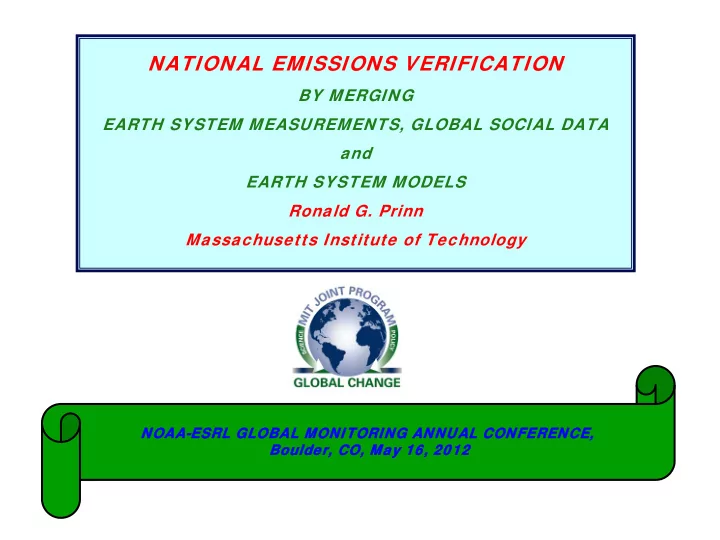
NATIONAL EMISSIONS VERIFICATION BY MERGING EARTH SYSTEM MEASUREMENTS, GLOBAL SOCIAL DATA and EARTH SYSTEM MODELS Ronald G. Prinn Massachusetts Institute of Technology NOAA-ESRL GLOBAL MONI NOAA-ESRL GLOBAL MONITORING ANNUAL CONFERENCE, TORING ANNUAL CONFERENCE, Boulder, CO, May 16, 2012 ulder, CO, May 16, 2012

TYPICAL CURRENT APPROACH Whether Whether Emission Emissi on Reductions Reductions are claimed are claimed through through Cap & Trade, Cap & Trade, Taxes, Taxes, or Mandates or Mandates Reliable Reliable Independent Independent Estimates Estimates y meas of of R meas Anthropogenic Anthropogenic y model Emissi Emissions ons =Ex of Greenhouse of Greenhouse Gases Gases are arguabl are arguably y u est u est ESSENTIAL ESSENTIAL P est P est

EXAMPLE: EXAMPLE: Advanced Gl Advanced Global obal Atmospheri Atmospheric Gases Experiment Gases Experiment INTERCOMPARISON WITH NOAA-GMD Ny-Alesund (Norway)

MA MAJOR JOR A AGAGE G GOA OAL SI SINC NCE I IT’S ’S 1978 S 1978 START: ESTIMATE FLOWS OF ESTIMATE FLOWS OF KYOTO & MONTREAL PROTOCOL GA KYOTO & MONTREAL PROTOCOL GASES USING SES USING ON SITE MEASU ON SITE MEASUREMEN EMENTS, TS, IN INVERSE METHODS, & G VERSE METHODS, & GLOBAL AL CIRCU CIRCULATION MO ATION MODEL DELS e. e.g. 28-level 1.8 g. 28-level 1.8 o x1.8 x1.8 o o or 2. or 2.8 o x2.8 x2.8 o o Model Model e. e.g. 28-level 1.8 g. 28-level 1.8 o x1.8 x1.8 o o or 2. or 2.8 o x2.8 x2.8 o o Model Model HI HIGH FREQUENCY MEAS GH FREQUENCY MEASUR UREMEN ENTS IN TS IN TH THE E for Atmospheric Transport & for Atmospheric T ransport & Chemis Chemistry try for Atmospheric T for Atmospheric Transport & ransport & Chemis Chemistry try BOUNDARY LAYER NEAR SOURCE REGI BOUNDARY LAYER NEAR S OURCE REGIONS ONS ARE ARE (MATCH or (MATCH or MOZART) MOZART) uses N uses NCEP & ECMWF EP & ECMWF (MATCH or (MATCH or MOZART) MOZART) uses N uses NCEP & ECMWF EP & ECMWF UNIQUE CO UNIQUE COMPONENTS IN THE GLOB MPONENTS IN THE GLOBAL AL meteorology meteorology MEASUREMENT NETWORK MEASUREMENT NETWORK meteorology meteorology e.g. Saikaw a, Thurs AM Talk on HCFC-22 inversions

HOW ACCURATE DO THE CIRCULATION MODELS NEED TO BE FOR INTERPRETING TRACE GAS OBSERVATIONS? e.g. SIMULATIONS OF CH 4 OBSERVATIONS DEMAND PRECISE INCLUSION OF EFFECTS OF w eather, ENSO, NAO, etc. (Chen & (Chen & Prinn, Prinn, J. Geophys. Res., J. Geophys. Res., 2005) 2005)

RECENT ADVANCE: RECENT ADVANCE: IMBEDDING HIGH IMBEDDING HIGH RESOLUTION RESOLUTION REGIONAL MODELS REGIONAL MODELS INTO A GLOBAL INTO A GLOBAL MODEL MODEL DEDUCED REGIONAL SF 6 EMISSIONS using AGAGE measurements and combined sensitivities from Eulerian MOZART (2.8 o x2.8 o , NCEP/NCAR) and Lagrangian NAME (0.38 o x0.56 o , UKMO) 3D models . Ref: Rigby Manning & Ref: Rigby Manning & Prinn, Atmos. Chem. Prinn, Phys., 2011 2011

LOOKING TO THE FUTURE LOOKING TO THE FUTURE Enhancing Understanding as w ell as Addressing Enhancing Understanding as w ell as Addressing Essential Needs to Verify Emission Reductions, Essential Needs to Verify Emission Reductions, Requires Requires Very Important Improvements in Current Capabilities Very Important Improvements in Current Capabilities Significant advances in the Global Observing System and Significant advances in the Global Observing System and Economic Data Collection System w ith close attention to Economic Data Collection System w ith close attention to Precision & Accuracy Precision & Accuracy For Greenhouse Gases: Higher time & Space Resolution; For Greenhouse Gases: Higher time & Space Resolution; GLOBAL measurements (SURFACE, PROFILES, MOLE FRACTIONS, GLOBAL measurements (SURFACE, PROFILES, MOLE FRACTIONS, FLUXES); ISOTOPIC Composition FLUXES); ISOTOPIC Composition (e.g. Rigby Tues Poster) (e.g. Rigby Tues Poster) Significant improvements in: Adjointed Models of Natural Significant improvements in: Adjointed Models of Natural Processes; Analysed Atmospheric & Oceanic Circulation; Processes; Analysed tmospheric & Oceanic Circulation; & Economic Emission Modeling & Economic Emission Modeling Estimation Models & Statistical Methods should Incorporate all Estimation Models & Statistical Methods should Incorporate all Reliable Information (w eighted by Precision and Accuracy) Reliable Information (w eighted by Precision and Accuracy)

Example current DATA AND Example current DATA AND OBSERVATIONS OBSERVATIONS ATMOSPHERIC GREENHOUSE GAS OBSERVATIONS Earth System Research Laboratory (NOAA-ESRL) Advanced Global Atmospheric Gases Experiment (AGAGE-NASA) Netw ork for Detection of Atmospheric Composition Change (NDACC) Scanning Imaging Absorption Spectrometer (SCIAMACHY-ESA) Greenhouse Gases Observing Satellite (GOSAT-Japan) Orbiting Carbon Observatory (OCO-NASA) Atmospheric Infrared Sounder (AIRS-NASA) Civil and Research aircraft (CARIBIC, HIPPO, ESRL flasks) NATURAL AND MANAGED LAND ECOSYSTEMS Net Fluxes of carbon from Tow ers (FLUXNET) International Long Term Ecological Research biomass netw ork (ILTER) Advanced Very High Resolution Radiometer (AVHRR) Moderate Resolution Imaging Spectro-radiometer (MODIS) OCEANS In situ measurements of CO 2 , nutrients, pH, chlorophyll, particles (GLODAP, CLIVAR, JGOFS, WOCE, BATS, HOT) Satellite derived products (SeaWifs, MODIS-Aqua, OCTS, chlorophyll) ECONOMICS DATASETS Economic Activity & Emission Factors (IEA, FAO, CDIAC, USGS, IRRI, IFA, CRF, UNFCC) Input/Output Data (EXIOPOL, WIOD, IDE, OECD)

STRATEGY FOR A STRATEGY FOR A Emissions Model Economic data GLOBAL GLOBAL Trade flows Emission model parameters OBSERVING OBSERVING Anthropogenic Atmospheric Carbon Transport Emissions SYSTEM FOR SYSTEM FOR CO2 , CH4 and Chemistry Model N2O VERIFICATION OF VERIFICATION OF agricultural land-use change ozone NATIONAL NATIONAL pCO 2 Ocean pCO 2 GREENHOUSE GAS GREENHOUSE GAS pN 2 O CO 2 + CO 2 + circulation pCH 4 N 2 O + N 2 O EMISSIONS EMISSIONS pN 2 O TEM CH 4 flux flux ( Terrestrial Carbon and Nitrogen Dynamics ) BioECCO VERIFYING leaf area index, ( Ocean Biogeochemistry ) EMISSION Atmospheric biomass change, circulation, eddy fluxes* PO 4 , O 2 , Fe, pCO 2 , REDUCTIONS FOR temperatures, dissolved inorganic carbon, fluxes GASES SUCH AS decomposition rate, alkalinity distributions vegetation C & N uptake, CO 2 , CH 4 & N 2 O dissolved microbial N uptake maximum growth rate, organic THAT HAVE gas transfer coefficient, carbon organic carbon rain ratio, in river SIGNIFICANT remineralization rate runoff NATURAL CLM ( Terrestrial Biogeophysics ) SOURCES & SINKS observations used KEY estimates from to constrain model models/observations surface temperature*, passive not actively coupled snow-water equivalent* control parameter within this framework AN “OPTIMAL” (s ee text ) * = no feedback, active constraint root uptake efficiency APPROACH USING coupling of active variables “NOTATION” OF CONTROL THEORY

STRATEGY FOR A GLOBAL OBSERVING SYSTEM FOR STRATEGY FOR A GLOBAL OBSERVING SYSTEM FOR VERIFICATION OF NATIONAL GREENHOUSE GAS EMISSIONS VERIFICATION OF NATIONAL GREENHOUSE GAS EMISSIONS VERIFYING EMISSION REDUCTIONS FOR ANTHROPOGENIC GASES SUCH AS CF 4 , SF 6 & CHF 3 AN “OPTIMAL” APPROACH USING CONTROL THEORY NOTATION Emissions Model Economic data Trade flows Emission model parameters Atmospheric Carbon Anthropogenic CFCs, HFCs, Transport and Chemistry Emissions PFCs, SF 6 Model GHG deposition GHG Atmospheric KEY observations used flux circulation, to constrain model temperatures, passive control parameter fluxes Ocean Transport and coupling of active variables Chemistry Model estimates from models/observations Gas transfer CFCs not actively coupled within this coeffecients framework (s ee text )

VARY CONTROLS U E (AND INITIAL CONDITIONS X E ( t = 0)) OF COUPLED SYSTEM, TO SEEK A SOLUTION OF THE COUPLED STATE X E ( t ), WHICH MINIMIZES THE OBJECTIVE FUNCTION J (Atmospheric, Terrestrial, Oceanic) . departure of initial state x E (0) from a first guess x E 0 ; model E ( t ) x E ( t ) minus observed y E ( t ) at time t deviation u E ( t) of the controls from a prior demand that x E ( t ) satisfy the model equations L E and the coupling functions M abcd (linking outputs of one model to inputs of another) through the introduction of Lagrange multipliers µ E (t) and µ abcd (t) .

Iterative minimization of modeled (red trajectory) vs. observed (blue dots) concentration misfit J , by variation of control variables. Optimal fit achieved for (n) , w hich lead to best estimate adjusted controls (parameters and emissions) u=u c (n) . concentrations x=x c Vary u C such as to minimize J (d J /du c = 0) via gradient- based optimizing algorithms (steepest descent, conjugate gradient, New ton method).