Multiple Comparisons Occasionally, e.g., at the start of a research - PowerPoint PPT Presentation
Lecture 7.1: Multiple Comparisons (A non-quiz topic) Examples of the need for multiple comparisons The problem with multiple comparisons post hoc; an outline of a solution Specific solutions: Fisher LSD, Tukey HSD, Holm (same as
Lecture 7.1: Multiple Comparisons (A ‘non-quiz’ topic) • Examples of the need for multiple comparisons • The problem with multiple comparisons post hoc; an outline of a solution • Specific solutions: Fisher LSD, Tukey HSD, Holm (same as False Discovery Rate, FDR), Dunn/ Bonferroni, Ryan (REGWQ) 1
Multiple Comparisons • Occasionally, e.g., at the start of a research project, we do not have a priori theories and contrasts and, therefore, cannot use the ‘surgical’ approach of planned comparisons . We simply want to see whether the different ‘ treatments ’ are all the same. • If the omnibus F ratio is significant , we may want to know after the fact (or post hoc ) which treatments seem to ‘ work ’ . This leads to multiple comparisons , e.g., (a) between every ‘ treatment ’ and the ‘ control ’ group ( k-1 comps), or (b) between every pair of ‘ treatments ’ ( k(k-1)/2 comps). 2
• Ex : Ss are randomly assigned to one of 3 conditions: No organiser (‘no.org’), Organiser before lecture (‘pre.org’), and Organiser after lecture (‘post.org’). • We might plan to examine 2 orthog contrasts, but we might also wish to compare ‘post’ with ‘no’, even though we have only 2 df between groups. some.no pre.post no.post no.org -2 0 -1 pre.org 1 -1 0 post.org 1 1 1 3
A Paw-Licking Example • Morphine (M) reduces a rat’s sensitivity to pain – under M for 1 st time, it takes them longer to lick their paws (signalling pain) when they are put on an uncomfortably warm surface. So ‘time to lick’ is also an index of M-tolerance (= 0 on 1 st trial). • Group MM receives M for 3 trials, then M on the critical 4 th trial in same lab setting. M-tolerance has developed, so RT is ‘normal’. • Group MS receives Saline on 4 th trial – they expected M but got S, so they are hypersensitive to pain and RT is very short. 4
A Paw-Licking Example • Group MM’ receives Morphine on 4 th trial, but in a different setting. The usual cues are absent on the 4 th trial, so rat shd not show M tolerance, and RT shd be long. • Group SM receives Saline for 3 trials and Morphine on 4 th trial, but in same setting. Rat shd not show M tolerance, and RT shd be long. • The 5 th group was SS. Predictions for RT are: SM = MM’ > MM ? SS > MS • Tr = M vs S on 1 st 3 trials; Test = M vs S on 4 th trial 5
A Paw-Licking Example Morphine Morphine Morphine Saline à à Saline à à à à à à à Saline Saline Morphine à Morphine Morphine (New Envt) Contrast 1 (new v same) Contrast 2 Tr: M v S Contrast 3 Test: M v S Contrast 4 Tr * Test Contrast 5 NA! (After Siegel, 1975 – See Howell, 6 th ed., p. 346)
Orthogonal contrasts for a (2x2 + 1) = 5-group design • The (train, test) groups in the ‘paw-lick’ study are MM, MS, SM, SS and MM’ (where M’ = M in a new context). The 1 st 4 groups conform to a tidy 2X2 design. Interpret each contrast below! Group l con l tr l te l T*T 1=MM 1 1 1 1 2=MS 1 1 -1 -1 3=SM 1 -1 1 -1 4=SS 1 -1 -1 1 5=MM’ -4 0 0 0 7
• Ex: ‘Paw-lick’ study of Morphine tolerance, with (train, test) groups, MM, MS, SM, SS, MM’ (where M’ = M in a new context; S = saline). The 1 st 4 groups conform to a tidy 2X2 design, and yields 3 orthog contrasts. But we might be interested also in comparing MM with MM’. Group l con l tr l te l T*T l Kara 1=MM 1 1 1 1 1 2=MS 1 1 -1 -1 0 3=SM 1 -1 1 -1 0 4=SS 1 -1 -1 1 0 5=MM’ -4 0 0 0 -1 8
The problem of Type I errors • Measure 10 variables on n = 100 Ss, and examine the correl matrix for sig correls. Assume true r = 0. How many observed r ’s do we expect to be sig (where | r | crit = 0.20 , p = .05)? (Ans. E = Np = 45*0.05 = 2.25. Why? ) • What is the P(at least 1 sig correl)? Ans . P(at least 1) = 1 – P(none) = 1 – (.95) 45 = .9. We’re almost certain to find at least 1 sig r ! This is the problem with multiple comarisons ! • Suppose we used α = .001 , instead of .05. | r | crit = 0.32 , and P(at least 1 sig r ) = 1 – (.999) 45 = .044, which is much more acceptable. 9
The problem of Type I errors • Decreasing the Type I error rate from .05 to α = . 001 , raises the critical value from 0.2 to | r | crit = 0.32 . • But then we would retain H 0 in cases of ‘seemingly large’ r , e.g., r = 0.27! That is, we would fail to detect violations of H 0 more often; i.e., our power would decrease . • How to decrease α without sacrificing too much power (assuming that sample size, n , is fixed)? • Recall that power depends on (i) α , (ii) the difference in parameter value (e.g., µ, ρ ) between H 0 and H 1 , and (iii) measurement error. 10
11
The classical approach to multiple comparisons relies on the concepts of Type I and Type II errors. False Discovery Rate (FDR) is a new approach to the multiple comparisons problem. Instead of controlling the chance of any false positives, i.e., Prob(at least 1 false positive) [as Bonferroni or other methods do], FDR controls the expected proportion of false positives among voxels that are judged to be suprathreshold. This turns out to be a relatively lenient metric for false positives, and it leads to an increase in power. The FDR approach is well-suited to the case of “many, many tests.” Later we will show how FDR thresholds are determined from the observed p-value distribution. 12
Outline of a Solution • To ensure that P(at least 1 sig r ) is acceptably low (e.g., .05 or .10), each individual test has to be done with a very stringent level of α (e.g., .01 or .001). • To proceed formally, let us label P(at least 1 sig r ) as the family-wise Type I error rate, α F ; α is, as before, the Type I error rate for each individual test . If we wish α F to be ‘small’ (e.g., .1), what should α be? If we set α at, e.g., .01, what is the resulting α F ? • In sum, what is the relationship between α F and α ? Which approaches ‘optimise’ this reln? 13
R packages, with examples • Most post-hoc comparisons fall into 1 of 2 categories. • Compare every ‘ treatment ’ to a ‘ control ’ group. Download with i nstall.packages( ‘ multcomp ’ ), and use Dunnett ’ s test. • Compare each treatment with every other treatment. Use TukeyHSD(model) and pairwise.t.test(score, group). • Other approaches include Fisher’s Least Significant Difference (LSD) approach, and the use of the False Discovery Rate (FDR). 14
Table 1: Mean outcome judgments as a function of Procedure (Voice vs No voice) and Outcome of Other Participant (Expt. 1) Outcome of other participant Dependent Variable Unknown Better Worse Equal Outcome satisfaction Voice 5.1 a,b 2.6 c 4.1 b 5.4 a No voice 3.1 d 2.8 c 4.2 b 5.3 a Outcome fairness Voice 5.1 b 2.3 c 2.0 c 6.1 a No voice 3.0 d 2.4 c,d 2.1 c 6.1 a Note: For each dependent variable , means with no subscripts in common differ significantly, as indicated by a least significant difference test for multiple comparisons between means (p < .05 ). 15
# Organiser study: Tukey HSD approach contrasts(d00$group, 2)=contr.treatment(3,base=2, contrasts=TRUE) rs3 = aov(score ~ group, data=d00) rs30 = TukeyHSD(rs3) print(rs30) [You may need to define a ‘group’ variable] Tukey multiple comparisons of means 95% family-wise confidence level Fit: aov(formula = score ~ group, data = d00) $group diff lwr upr p adj pre.org-no.org 0.1 -1.57075607 1.770756 0.9879376 post.org-no.org 1.7 0.02924393 3.370756 0.0455236 post.org-pre.org 1.6 -0.07075607 3.270756 0.0624878 16
• plot(rs30) 17
# Organiser study: Holm’s approach rs31 = pairwise.t.test(d00$score, d00$group) print(rs31) Pairwise comparisons using t tests with pooled SD data: d00$score and d00$group no.org pre.org pre.org 0.883 - post.org 0.054 0.054 P value adjustment method: holm (Holm ’ s procedure for controlling the familywise Type I error rate will be introduced in a later slide.) 18
Error Rates in Multiple Hypothesis Testing • For a single test of a null hypothesis, H 0 , α • = P(Reject H 0 | H 0 true), the Type I error rate, and β • = P(Retain H 0 | H 0 false), the Type II error rate β • Power = 1 - • How to define “ error rate ” when we test m hypotheses simultaneously? 19
Decision Retain Reject True Correct False Alarm H 0 Retention Type I error False Miss Correct Type II error Rejection False Alarm aka False Discovery or False Rejection. Miss aka False Non-Discovery α = False Alarm rate = P(Reject H 0 |H 0 True) β β = P(Retain H 0 |H 0 False); 1 - = Power 20
Testing m null hypotheses • If we test the (45) correlations among 10 α variables for significance, with = .05, we wd expect about 5% of them, i.e., about 2 or 3 r ’ s to be significant, even if H 0 is true everywhere ; and the prob of at least 1 False Alarm wd be much greater than 0.05. • The prob of at least 1 Type I error when testing m null hypotheses is called the α F familywise Type I error rate , . What is α α F the relation between and ? 21
Recommend
More recommend
Explore More Topics
Stay informed with curated content and fresh updates.
