Motivation Argumentation is the support of (or a reason for) one - PowerPoint PPT Presentation

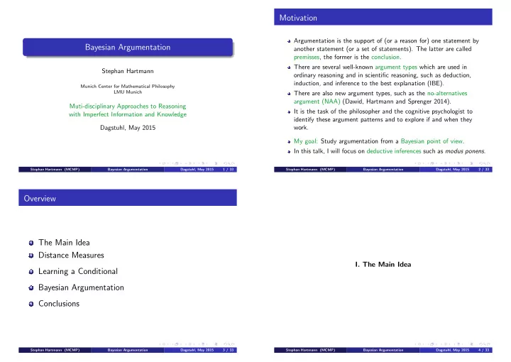
Motivation Argumentation is the support of (or a reason for) one statement by Bayesian Argumentation another statement (or a set of statements). The latter are called premisses, the former is the conclusion. There are several well-known argument types which are used in Stephan Hartmann ordinary reasoning and in scientific reasoning, such as deduction, induction, and inference to the best explanation (IBE). Munich Center for Mathematical Philosophy LMU Munich There are also new argument types, such as the no-alternatives argument (NAA) (Dawid, Hartmann and Sprenger 2014). Muti-disciplinary Approaches to Reasoning It is the task of the philosopher and the cognitive psychologist to with Imperfect Information and Knowledge identify these argument patterns and to explore if and when they Dagstuhl, May 2015 work. My goal: Study argumentation from a Bayesian point of view. In this talk, I will focus on deductive inferences such as modus ponens . Stephan Hartmann (MCMP) Bayesian Argumentation Dagstuhl, May 2015 1 / 33 Stephan Hartmann (MCMP) Bayesian Argumentation Dagstuhl, May 2015 2 / 33 Overview 1 The Main Idea 2 Distance Measures I. The Main Idea 3 Learning a Conditional 4 Bayesian Argumentation 5 Conclusions Stephan Hartmann (MCMP) Bayesian Argumentation Dagstuhl, May 2015 3 / 33 Stephan Hartmann (MCMP) Bayesian Argumentation Dagstuhl, May 2015 4 / 33

Deductive Inferences Two Issues Consider the following argument: P1: It currently rains in Munich. 1 The information (i.e. the premisses of the argument) may come from P2: If it rains, then the streets get wet. a source which we do not fully trust. ————————————————– We may have listened to the weather forecast and the weather forecast C: Munich’s Ludwigstraße is currently wet. does not say that it will rain. Someone might have told us and we are not sure how reliable this People familiar with formal logic represent the argument as an person is. instance of modus ponens . . . . A 2 Disabling conditions may come to mind. A → B The street might be covered by something which prevents it from —————– becoming wet. B There might be strong winds in which case the rain does not have a chance to hit the ground. We say that the conclusion follows with necessity, and that we make a . . . mistake if we do not infer B. We ask: Are there other (rational) ways of reasoning with these premisses? Stephan Hartmann (MCMP) Bayesian Argumentation Dagstuhl, May 2015 5 / 33 Stephan Hartmann (MCMP) Bayesian Argumentation Dagstuhl, May 2015 6 / 33 Upshot The Main Idea – A Sketch 1 The agent entertains the propositions A, B,. . . 2 The agent represents the causal relations between these propositions in a causal (“Bayesian”) network. Taking these concerns into account may lead a rational agent to 3 The agent has prior beliefs about the propositions A, B,. . . which are arrive at a different conclusion. represented by a probability distribution P . We therefore construct a fully Bayesian theory of argumentation 4 The agent learns new information (i.e. the agent learns the premisses which is, or so we hope, in line with how real people reason and which of the argument) and represents them as constraints on the posterior makes nevertheless sense from a normative point of view. distribution. The theory can be tested and it allows for some flexibility. (What I This is really the key of my proposal: argumentation = learning present here are only the first steps of a research program.) 5 The agent then determines the posterior distribution P ′ by minimizing some “distance” measure (such as the Kullback Leibler divergence) between P ′ and P . Intuitive idea: we want to change our beliefs in a conservative way. Stephan Hartmann (MCMP) Bayesian Argumentation Dagstuhl, May 2015 7 / 33 Stephan Hartmann (MCMP) Bayesian Argumentation Dagstuhl, May 2015 8 / 33

The Kullback-Leibler Divergence Let S 1 , . . . , S n be the possible values of a random variable S over which probability distributions P and P ′ are defined. The Kullback-Leibler divergence between P ′ and P is then given by n P ′ ( S i ) log P ′ ( S i ) II. Distance Measures � D KL ( P ′ || P ) := P ( S i ) . i =1 Note that the KL divergence is not symmetrical. So it is not a distance. Note also that if the old distribution P is the uniform distribution, then minimizing the Kullback-Leibler divergence amounts to maximizing the entropy. Stephan Hartmann (MCMP) Bayesian Argumentation Dagstuhl, May 2015 9 / 33 Stephan Hartmann (MCMP) Bayesian Argumentation Dagstuhl, May 2015 10 / 33 Alternative Measures Applications To find the new probability distribution P ′ , one minimizes D KL ( P ′ || P ) Here is an alternative measure: making sure that specific constraints are satisfied. n 1 Condtionalization P ( S i )) 2 . � � � D ( P ′ || P ) := ( P ′ ( S i ) − Constraint: P ′ ( E ) = 1 i =1 2 Jeffrey Conditionalization Interestingly, it gives the same results for many of the cases we Constraint: P ′ ( E ) = e ′ < 1 studied. But not for all. 3 Learning the conditional A → B I consider it to be (at least partly) an empirical question which measure is best and it would be interesting to run experiments on this. Constraint: P ′ ( B | A ) = 1 Stephan Hartmann (MCMP) Bayesian Argumentation Dagstuhl, May 2015 11 / 33 Stephan Hartmann (MCMP) Bayesian Argumentation Dagstuhl, May 2015 12 / 33

Learning a Conditional: The General Recipe Indicative conditionals typically show up in the premisses of a deductive argument, and so we have to understand how learning a conditional works. If one learns the conditional A → B, then the new distribution P ′ has to satisfy the constraint P ′ ( B | A ) = 1 III. Learning a Conditional the causal structure of the problem at hand has to be specified in a causal network. the new distribution P ′ should be as close as possible to the old distribution, satisfying all constraints. One option here is to use the Kullback-Leibler divergence. If one does this, one can meet a number of challenges presented by Douven and others. Stephan Hartmann (MCMP) Bayesian Argumentation Dagstuhl, May 2015 13 / 33 Stephan Hartmann (MCMP) Bayesian Argumentation Dagstuhl, May 2015 14 / 33 The Ski Trip Example The Ski Trip Example Harry sees his friend Sue buying a skiing outfit. This surprises him a bit, Harry sees his friend Sue buying a skiing outfit. This surprises him a bit, because he did not know of any plans of hers to go on a skiing trip. He because he did not know of any plans of hers to go on a skiing trip. He knows that she recently had an important exam and thinks it unlikely that knows that she recently had an important exam and thinks it unlikely that she passed. Then he meets Tom, his best friend and also a friend of Sue, she passed. Then he meets Tom, his best friend and also a friend of Sue, who is just on his way to Sue to hear whether she passed the exam, and who is just on his way to Sue to hear whether she passed the exam, and who tells him, who tells him, If Sue passed the exam, then her father will take her on a skiing vacation. If Sue passed the exam, then her father will take her on a skiing vacation. Recalling his earlier observation, Harry now comes to find it more likely that Sue passed the exam. Ref.: Douven and Dietz (2011) Stephan Hartmann (MCMP) Bayesian Argumentation Dagstuhl, May 2015 15 / 33 Stephan Hartmann (MCMP) Bayesian Argumentation Dagstuhl, May 2015 15 / 33

Modeling the Ski Trip Example The Ski Trip Example We define three variables: Learning: P ′ ( B ) = 1 and P ′ ( S | E ) = 1. E: Sue has passed the exam. Again, the causal structure does not change. S: Sue is invited to a ski vacation. B: Sue buys a ski outfit. Theorem: Consider the Bayesian Network above with the prior probability distribution. Let The causal structure is given as follows: p 1 p 2 k 0 := . E S B q 1 p 2 + q 1 q 2 We furthermore assume that (i) the posterior probability distribution P ′ is defined over the same Bayesian Network, (ii) the learned Additionally, we set P ( E ) = e and information is modeled as constraints on P ′ , and (iii) P ′ minimizes P ( S | E ) = p 1 , P ( S |¬ E ) = q 1 the Kullback-Leibler divergence to P. Then P ′ ( E ) > P ( E ) , iff k 0 > 1 . P ( B | S ) = p 2 , P ( B |¬ S ) = q 2 . The same result obtains for the material conditional. Note that the story suggests that p 1 > q 1 and p 2 > q 2 . Stephan Hartmann (MCMP) Bayesian Argumentation Dagstuhl, May 2015 16 / 33 Stephan Hartmann (MCMP) Bayesian Argumentation Dagstuhl, May 2015 17 / 33 The Ski Trip Example: Assessing k 0 The Ski Trip Example: Assessing k 0 1 Harry thought that it is unlikely that Sue passed the exam, hence e is small. 2 Harry is surprised that Sue bought a skiing outfit, hence We conclude that P ( B ) = e ( p 1 p 2 + p 1 q 2 ) + e ( q 1 p 2 + q 1 q 2 ) is small. p 1 p 2 k 0 : = 3 As e is small, we conclude that q 1 p 2 + q 1 q 2 := ǫ is small. q 1 p 2 + q 1 q 2 p 1 4 p 2 is fairly large ( ≈ 1), because Harry did not know of Sue’s plans to = ǫ · p 2 go skiing, perhaps he even did not know that she is a skier. And so it is very likely that she has to buy a skiing outfit to go on the skiing will typically be greater than 1. Hence, P ′ ( E ) > P ( E ). trip. 5 At the same time, q 2 will be very small as there is no reason for Harry to expect Sue to buy such an outfit in this case. 6 p 1 may not be very large, but the previous considerations suggest that p 1 ≫ ǫ . Stephan Hartmann (MCMP) Bayesian Argumentation Dagstuhl, May 2015 18 / 33 Stephan Hartmann (MCMP) Bayesian Argumentation Dagstuhl, May 2015 19 / 33