Motivation systemfit systemfit Many theoretical models consist of - PowerPoint PPT Presentation

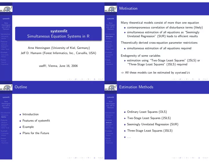
Motivation systemfit systemfit Many theoretical models consist of more than one equation Arne Arne Henningsen Henningsen contemporaneous correlation of disturbance terms (likely) and Jeff D. and Jeff D. Hamann Hamann systemfit simultaneous estimation of all equations as “Seemingly Introduction Introduction Simultaneous Equation Systems in R Unrelated Regression” (SUR) leads to efficient results Motivation Motivation Outline Outline Features Features Theoretically derived cross-equation parameter restrictions Methods Methods Estimation Estimation Arne Henningsen (University of Kiel, Germany) Control Control simultaneous estimation of all equations required Other Tools Other Tools Example Jeff D. Hamann (Forest Informatics, Inc., Corvallis, USA) Example Commands Commands Endogeneity of some variables Output Output Future Future estimation using “Two-Stage Least Squares” (2SLS) or General General “Three-Stage Least Squares” (3SLS) required Arguments Arguments useR!, Vienna, June 16, 2006 ⇒ All these models can be estimated by systemfit Outline Estimation Methods systemfit systemfit Arne Arne Henningsen Henningsen and Jeff D. and Jeff D. Hamann Hamann Ordinary Least Squares (OLS) Introduction Introduction Introduction Motivation Motivation Outline Outline Two-Stage Least Squares (2SLS) Features of systemfit Features Features Methods Methods Seemingly Unrelated Regression (SUR) Estimation Estimation Control Control Example Other Tools Other Tools Three-Stage Least Squares (3SLS) Example Example Plans for the Future Commands Commands Output Output . . . Future Future General General Arguments Arguments

Estimation Control Other Tools systemfit systemfit Arne Arne Henningsen Henningsen and Jeff D. and Jeff D. Hamann Hamann imposition of linear restrictions Introduction Introduction systemfitClassic : wrapper function for (classical) instrumental variables Motivation Motivation panel-like data in long format Outline Outline Features Features iteration of FGLS estimation Methods Methods testing linear hypotheses using the F-, Wald-, and Estimation Estimation Control Control LR-statistic formulas for the residual covariance matrix Other Tools Other Tools Example Example Hausman test for the consistency of the 3SLS estimator Commands formulas for 3SLS estimation Commands Output Output Future Future . . . General General Arguments Arguments Example: Commands Results of the Entire System systemfit systemfit systemfit results method: SUR Arne Arne Henningsen Henningsen and Jeff D. and Jeff D. from Kmenta (1986): Elements of Econometrics, p. 685 Hamann Hamann N DF SSR MSE RMSE R2 Adj R2 demand 20 17 65.6829 3.86370 1.96563 0.755019 0.726198 specification of the equation system: Introduction Introduction supply 20 16 104.0584 6.50365 2.55023 0.611888 0.539117 Motivation Motivation eqDemand <- consump ~ price + income Outline Outline Features eqSupply <- consump ~ price + farmPrice + trend Features [...] Methods Methods eqSystem <- list(demand=eqDemand, supply=eqSupply) Estimation Estimation Control Control Other Tools Other Tools The correlations of the residuals estimation using method “SUR”: Example Example demand supply Commands Commands fitsur <- systemfit("SUR", eqSystem, data=Kmenta) Output Output demand 1.000000 0.982348 Future Future supply 0.982348 1.000000 printing summary results: General General Arguments Arguments summary( fitsur ) The determinant of the residual covariance matrix: 0.879285 OLS R-squared value of the system: 0.683453 McElroy’s R-squared value for the system: 0.788722

Results of a Single Equation Plans for the Future systemfit systemfit Arne Arne SUR estimates for ’demand’ (equation 1) estimation with unbalanced data sets Henningsen Henningsen Model Formula: consump ~ price + income and Jeff D. and Jeff D. Hamann Hamann estimation methods: LIML, FIML, and GMM Estimate Std. Error t value Pr(>|t|) Introduction Introduction Motivation Motivation fitting equation systems with serially correlated and (Intercept) 99.332894 7.514452 13.218913 0 *** Outline Outline price -0.275486 0.088509 -3.112513 0.006332 ** heteroscedastic disturbances Features Features Methods income 0.29855 0.041945 7.117605 2e-06 *** Methods Estimation Estimation spatial econometric methods Control Control --- Other Tools Other Tools Signif. codes: 0 ’***’ 0.001 ’**’ 0.01 ’*’ 0.05 ’.’ 0.1 ’ Example Example simplify specification of parameter restrictions Commands Commands Output Output Residual standard error: 1.96563 on 17 degrees of freedom Future Future improving the function nlsystemfit to estimate systems Number of observations: 20 Degrees of Freedom: 17 General General of non-linear equations Arguments Arguments SSR: 65.682902 MSE: 3.8637 Root MSE: 1.96563 Multiple R-Squared: 0.755019 Adjusted R-Squared: 0.726198 . . . User Interface: Arguments Arguments systemfit systemfit Arne Arne Henningsen Henningsen and Jeff D. and Jeff D. Arguments of systemfit : Hamann Hamann Reducing arguments? formula3sls q.restr method Introduction Introduction Motivation Motivation R.restr method probdfsys TX eqns Outline Outline Features Features q.restr eqns single.eq.sigma maxiter eqnlabels Methods Methods Estimation Estimation TX inst Control tol solvetol Control inst Other Tools Other Tools control (like in optim ) data rcovformula saveMemory Example data Example Commands Commands Output centerResiduals (more in the future) Output R.restr However: This would break existing code! Future Future General General Arguments Too many? Arguments

The End . . . systemfit Arne Henningsen and Jeff D. Hamann Introduction Motivation Outline Thank you for your attention! Features Methods Estimation Control Other Tools Example Commands Output Future General Arguments