Feature Extraction Aleix M. Martinez aleix@ece.osu.edu Continuous - PDF document

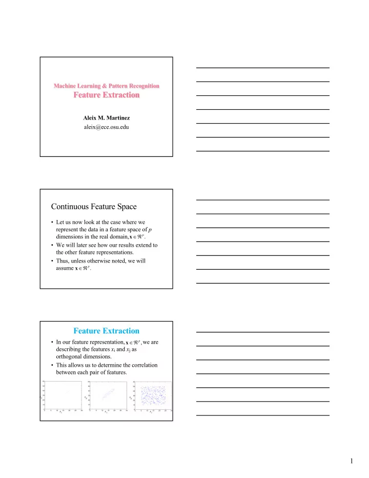
Machine Learning & Pattern Recognition Feature Extraction Aleix M. Martinez aleix@ece.osu.edu Continuous Feature Space • Let us now look at the case where we represent the data in a feature space of p Î Â dimensions in the real domain, p x . • We will later see how our results extend to the other feature representations. • Thus, unless otherwise noted, we will assume Î Â p x . Feature Extraction • In our feature representation, we are Î Â p x , describing the features x i and x j as orthogonal dimensions. • This allows us to determine the correlation between each pair of features. 1

Correlations • Linear correlations (or co-relations) translates to a linear relationship between variables. • If x i1 and x i2 are linearly dependent, we can write x i2 = f ( x i1 ), where f (.) is linear. • Ex: • If they are not 100% correlated, we have Error function. Linear least-squares • Our error function is a set of homogenous equations: with n > p . • We can rewrite these as Xa = 0. • If rank( X )= p , there is a unique solution. • When rank( X )> p , R 2 >0. Then, to minimize R 2 , we need to minimize ( Xa ) 2 = a T X T Xa . That is: we want to find the dimension in R p where the data has largest variance . • Let Q = X T X . And assume . We can then write = l a T Qa . symmetric, positive semidefinite matrix ( ) . = • Now, let We have: A a , ! , a 1 p A T = L QA . Schur decomposition 2

Eigenvalue decomposition • Since the columns of A define an orthogonal bases, i.e., A T A = I , we can write = A L QA . • This is the well-known eigenvalue decomposition equation. ( ) , L = l ! l • In the equations above diag , , 1 p l ³ ³ l ³ and we assume ! 0 . 1 p 3