Moral Hazard vs. Liquidity and Optimal Unemployment Insurance Raj - PowerPoint PPT Presentation
Moral Hazard vs. Liquidity and Optimal Unemployment Insurance Raj Chetty UC-Berkeley and NBER April 2008 MOTIVATION Classic empirical result: Unemployment insurance (UI) increases unemployment durations 10% inc. in UI 4-8% increase in
Moral Hazard vs. Liquidity and Optimal Unemployment Insurance Raj Chetty UC-Berkeley and NBER April 2008
MOTIVATION • Classic empirical result: Unemployment insurance (UI) increases unemployment durations 10% inc. in UI 4-8% increase in durations (Moffitt 1985, Meyer 1990) • • Traditional interpretation of this result: moral hazard caused by substitution effect: Agents perceive wage as w-b, not w • Krueger and Meyer (2002): Temporary benefits “lead to short-run variation in wages with mostly a substitution effect” • Feldstein (2005): “Existing programs have substantial undesirable effect on incentives.…UI programs raise unemployment.” • This paper: 1. Shows that 60% of the effect of UI benefits on durations is due to a “liquidity effect,” not moral hazard using data from the U.S. 2. Develops a new method of characterizing optimal UI benefit level using this evidence
CONSUMPTION SMOOTHING AND LIQUIDITY EFFECT • Analysis motivated by evidence that many job losers cannot smooth consumption fully due to failures in credit and insurance markets • Gruber (1997), Browning and Crossley (2001): UI benefits raise consumption while unemployed, particularly for those without assets • Median liquid wealth net of unsecured debt for job losers is $163 • Borrowing difficult for those without jobs • When households cannot smooth perfectly, UI benefits also affect search behavior through a liquidity effect • Higher benefits more consumption when unemployed less pressure to find a job quickly longer duration • This is independent of any moral hazard effect: not a response to distorted prices.
LIQUIDITY VS. MORAL HAZARD: WELFARE IMPLICATIONS • Distinction between moral hazard and liquidity of interest because of implications for optimal policy to correct credit/insurance market failures • Substitution effect: socially suboptimal response to wedge between social and private marginal product of labor (w vs. w-b) lower welfare • Liquidity effect: response to the correction of a market failure (imperfect credit and insurance markets) higher welfare
“EXACT IDENTIFICATION” APPROACH TO WELFARE ANALYSIS • I develop a new formula for the optimal level of UI benefits in terms of the magnitude of the liquidity effect relative to moral hazard • Formula is “exactly identified” and does not require estimation of primitives, in contrast with standard “structural” method Less model-dependent and more empirically credible results • I implement formula by estimating liquidity and moral hazard effects using variation in UI benefit levels and severance payments
OUTLINE I) Job search model and formula for optimal benefit level II) Evidence on the role of liquidity constraints in the UI-duration link III) Evidence on severance pay and durations IV) Calibration of welfare gain from UI V) Followup study: Card, Chetty, and Weber (2007)
SEARCH MODEL: SETUP • Discrete time model with finite planning horizon T • Interest rate and discount rate equal to 0 • Individual loses job in period t = 0 • Let u(c t ) denote utility over consumption • Dynamic budget constraint: A t+1 = A t + y t - c t Asset limit: A t ≥ • L • Assumptions in baseline case: 1. Assets prior to job loss exogenous 2. No heterogeneity 3. Fixed wages: choose only search intensity, not reservation wage
JOB SEARCH • If unemployed in period t, worker first chooses search intensity s t • Finds a job that begins immediately in period t with probability s t e . Jobs are permanent, pay wage w t – . • If job found, consumes c t • If no job found: receives benefit b t , consumes c t u , enters t+1 unemployed c t e = c t+1 e = … s t Period t s t+1 c t+1 e 1-s t c t u 1-s t+1 c t+1 u Cost of job search: (s t • )
• Value function for agent who finds a job in period t : V t A t max A t 1 ≥ L v A t − A t 1 w t − V t 1 A t 1 • Value function for agent who does not find a job in period t : U t A t max A t 1 ≥ L u A t − A t 1 b t J t 1 A t 1 where J(A t+1 ) is value of entering next period unemployed. • Agent chooses s t to maximize expected utility: J A t max s t s t V t A t 1 − s t U t A t − s t • First order condition for optimal search intensity: ′ s t ∗ V t A t − U t A t
MORAL HAZARD VS. LIQUIDITY • Effect of benefits on durations: ∂ s t / ∂ b t − u ′ c t u / ′′ s t • Benefit effect can be decomposed into two conceptually distinct terms: ∂ s t / ∂ A t v ′ c t e − u ′ c t u / ′′ s t ≤ 0 ∂ s t / ∂ w t v ′ c t e / ′′ s t 0 ∂ s t / ∂ b t ∂ s t / ∂ A t − ∂ s t / ∂ w t Liquidity Moral Hazard (subst. effect) • No liq. effect for agents who smooth perfectly; negligible liq. effect for those who are not credit constrained because unemp. shocks small • Liquidity and total benefit effects large for agents who cannot smooth relative to permanent income (e.g. low asset, credit constrained)
Figure 1 UI Benefit and Liquidity Effects by Initial Assets Benefits b paid for 26 wks. Horizon T = 500 wks. Probability of finding a job in period 0 ( s 0 ) Asset Limit L = -$1,000 Mean Dur (b=0.5w) = 16 wks. s 0 (b;A 0 = -$1000) s 0 (a;A 0 = -$1000) s 0 (a;A 0 =$13,000) s 0 (b,A 0 =$13,000) Benefit or Annuity Level (a,b)
WELFARE ANALYSIS: OPTIMAL UI BENEFITS • Social planner’s problem: find policy that maximizes expected utility given failures in credit and insurance markets • Restrict attention here to constant-benefit, fixed duration UI policies: pay a benefit b for B periods. Take B as exogenous (B = 26 in U.S.). • Let D denote expected unemployment duration and D B denote expected duration on UI system • Planner solves: max b , J 0 b , s.t. D B b T − D • I derive a formula for the optimal benefit level b* in terms of the liquidity and moral hazard effects
DERIVATION OF FORMULA IN STATIC MODEL (T = 1) • Planner’s objective when B = T = 1: W b 0 1 − s 0 b 0 u A 0 b 0 s 0 b 0 v A 0 w 0 − − s 0 b 0 max b 0 s.t. b 0 1 − s 0 b 0 s 0 b 0 • Welfare gain from increasing b by $1 is e d db 0 1 − s 0 u ′ c 0 u − s 0 v ′ c 0 dW db 0 • Lucas-type money metric: welfare gain relative to $1 increase in wage u ′ c 0 u − v ′ c 0 e − 1 − s , b e 1 − s 0 db 0 dW dW db 0 / s 0 v ′ c 0 s 0 v ′ c 0 s 0 e − 1 − s , b 1 − s 0 −∂ s 0 / ∂ A 0 s 0 s 0 ∂ s 0 / ∂ w 0
GENERAL FORMULA FOR OPTIMAL BENEFITS • General case: DB , b 1 − D B db ≃ D R − dW where R is the liquidity/MH ratio and is fraction of time employed : ∂ s 0 − B ∂ A 0 T − D R and B ∂ s 0 ∂ A 0 − ∂ s 0 T ∂ b • This formula gives marginal welfare gain at a point b. • To test whether a given level b is optimal, estimate moral hazard and liquidity effects around that level and check if dW(b)/db = 0 • Some implications: Liquidity effect 0 optimal benefit is 0. • • Larger elasticity does not imply lower opt. ben.
EXTENSIONS: THEORETICAL ROBUSTNESS • Same formula holds when we allow for: 1. Endogenous asset choice prior to job loss: A 0 responds to b 2. Endogenous private insurance: private/informal insurance contract chosen prior to job loss responds to b 3. Stochastic wages (caveat about measurement of search intensity) 4. Heterogeneity: formula yields mean per-capita welfare gain • Reason for robustness: Envelope conditions eliminate first-order effects of other behaviors on marginal utilities that matter for welfare. • Changes in model affect dW/db only through the key parameters that enter the formula.
INTUITION FOR TEST Formula is a “revealed preference” approach to valuing insurance • Infer value of UI to agent by observing what he would do if money given as a cash-grant without distorted incentives • If agent would not use money to extend duration, infer that only takes longer because of price subsidy (moral hazard) • But if he uses cash grant to extend duration, indicates that UI facilitates a choice he would make if markets were complete • Same strategy can be used in valuing other types of insurance, such as health, disability, etc. • Make inferences from agent’s choices instead of directly computing costs and benefits of the policy • Key assumption: Agents optimize fully, so their actions when incentives are not distorted reveals social optimum
Recommend
More recommend
Explore More Topics
Stay informed with curated content and fresh updates.
