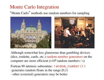
Monte Carlo Integration for Image Synthesis Adapted from Thomas - PowerPoint PPT Presentation
Monte Carlo Integration for Image Synthesis Adapted from Thomas Funkhouser Princeton University C0S 526, Fall 2002 Main Sources Books Realistic Ray Tracing, Peter Shirley Realistic Image Synthesis Using Photon Mapping,
Monte Carlo Integration for Image Synthesis Adapted from… Thomas Funkhouser Princeton University C0S 526, Fall 2002
Main Sources • Books � Realistic Ray Tracing, Peter Shirley � Realistic Image Synthesis Using Photon Mapping, Henrik Wann Jensen � Advanced Global Illumination, Dutre, Bekaert & Bala • Theses � Robust Monte Carlo Methods for Light Transport Simulation, Eric Veach � Mathematical Models and Monte Carlo Methods for Physically Based Rendering, Eric La Fortune • Course Notes � Mathematical Models for Computer Graphics, Stanford, Fall 1997 � State of the Art in Monte Carlo Methods for Realistic Image Synthesis, Course 29, SIGGRAPH 2001
Outline • Motivation • Monte Carlo integration • Monte Carlo path tracing • Variance reduction techniques • Sampling techniques • Conclusion
Motivation • Rendering = integration � Antialiasing � Soft shadows � Indirect illumination � Caustics
Motivation • Rendering = integration � Antialiasing � Soft shadows Eye � Indirect illumination � Caustics Pixel x P � = → L L(x e) dA Surface S
Motivation • Rendering = integration Light � Antialiasing x ’ � Soft shadows Eye � Indirect illumination � Caustics x Surface � � ( , ′ , ) ′ ( , ′ ) ( , ′ ) = → + → → → L(x, w ) L (x,x e) f x x x x e L( x x)V x x G x x dA e r S
Motivation • Rendering = integration � Antialiasing � Soft shadows � Indirect illumination � Caustics Herf � � ( , ′ , ) ′ ( , ′ ) ( , ′ ) = → + → → → L(x, w ) L (x,x e) f x x x x e L( x x)V x x G x x dA e r S
Motivation • Rendering = integration Surface � Antialiasing Light � Soft shadows Eye � Indirect illumination � Caustics ω ω ’ x Surface � � � � � � � � � ( , ′ , ) ′ ( ′ ) = + • L (x, w ) L (x, w ) f x w w L (x, w ) w n d w o e r i Ω
Motivation • Rendering = integration � Antialiasing � Soft shadows � Indirect illumination � Caustics Debevec � � � � � � � � � ( , ′ , ) ′ ( ′ ) = + • L (x, w ) L (x, w ) f x w w L (x, w ) w n d w o e r i Ω
Motivation Specular • Rendering = integration Surface Light � Antialiasing � Soft shadows Eye � Indirect illumination � Caustics ω ω ’ x Diffuse Surface � � � � � � � � � ( , ′ , ) ′ ( ′ ) = + • L (x, w ) L (x, w ) f x w w L (x, w ) w n d w o e r i Ω
Motivation • Rendering = integration � Antialiasing � Soft shadows � Indirect illumination � Caustics Jensen � � � � � � � � � ( , ′ , ) ′ ( ′ ) = + • L (x, w ) L (x, w ) f x w w L (x, w ) w n d w o e r i Ω
Challenge • Rendering integrals are difficult to evaluate � Multiple dimensions � Discontinuities » Partial occluders » Highlights » Caustics Drettakis � � ( , ′ , ) ′ ( , ′ ) ( , ′ ) = → + → → → L(x, w ) L (x,x e) f x x x x e L( x x)V x x G x x dA e r S
Challenge • Rendering integrals are difficult to evaluate � Multiple dimensions � Discontinuities » Partial occluders » Highlights » Caustics Jensen � � ( , ′ , ) ′ ( , ′ ) ( , ′ ) = → + → → → L(x, w ) L (x,x e) f x x x x e L( x x)V x x G x x dA e r S
Outline • Motivation • Monte Carlo integration • Monte Carlo path tracing • Variance reduction techniques • Sampling techniques • Conclusion
Slide courtesy of Integration in 1D Peter Shirley 1 � ( ) ? = f x dx 0 f(x) x=1
Slide courtesy of We can approximate Peter Shirley 1 1 � � ( ) ( ) = f x dx g x dx 0 0 g(x) f(x) x=1
Slide courtesy of Or we can average Peter Shirley 1 � ( ) ( ( )) = f x dx E f x 0 f(x) E(f(x)) x=1
Slide courtesy of Estimating the average Peter Shirley 1 1 N � � ( ) ( ) = f x dx f x i N 1 = i 0 f(x) E(f(x)) x 1 x N
Slide courtesy of Other Domains Peter Shirley b − b a N � � ( ) ( ) = f x dx f x i N 1 = i a f(x) < f > ab x=a x=b
Multidimensional Domains • Same ideas apply for integration over … � Pixel areas 1 � Surfaces N � � ( ) ( ) = f x dx f x � Projected areas i N = 1 i UGLY � Directions Eye � Camera apertures � Time Pixel � Paths x Surface
Outline • Motivation • Monte Carlo integration • Monte Carlo path tracing • Variance reduction techniques • Sampling techniques • Conclusion
Monte Carlo Path Tracing Specular • Integrate radiance Surface for each pixel Light by sampling paths randomly Eye Pixel x Diffuse Surface � � � � � � � � � ′ ′ ′ ( , , ) ( ) = + • L (x, w ) L (x, w ) f x w w L (x, w ) w n d w o e r i Ω
Pixel Sampling
Simple Stochastic Ray Tracing
Radiance Sampling • Monte Carlo approximation • but RHS has unknowns
Simple Monte Carlo Path Tracer Step 1: Choose a ray (x, y), (u, v), t; weight = 1 • Step 2: Trace ray to find intersection with nearest surface • Step 3: Randomly decide whether to • compute emitted or reflected light Step 3a: If emitted, • return weight * Le Step 3b: If reflected, • weight *= reflectance • Generate ray in random direction • Go to step 2 •
A Simple Algorithm
Monte Carlo Path Tracing • Advantages � Any type of geometry (procedural, curved, ...) � Any type of BRDF (specular, glossy, diffuse, ...) � Samples all types of paths (L(SD)*E) � Accuracy controlled at pixel level � Low memory consumption � Unbiased - error appears as noise in final image • Disadvantages � Slow convergence � Noise in final image
Monte Carlo Path Tracing Big diffuse light source, 20 minutes Jensen
Monte Carlo Path Tracing 1000 paths/pixel Jensen
Variance N [ ] = � ( ( )) [ ( ) ( ( ))] 2 i − Var E f x f x E f x = 1 i E(f(x)) x 1 x N
Variance 1 [ ] [ ] ( ( )) ( ) = Var E f x Var f x N Variance decreases with 1/N Error decreases with 1/sqrt(N) E(f(x)) x 1 x N
Outline • Motivation • Monte Carlo integration • Monte Carlo path tracing • Variance reduction techniques • Sampling techniques • Conclusion
Variance • Problem: variance decreases with 1/N More samples More samples removes noise removes noise SLOWLY SLOWLY E(f(x)) x 1 x N
Variance Reduction Techniques • Importance sampling • Stratified sampling • Metropolis sampling • Quasi-random 1 1 N � � ( ) ( ) = f x dx f x i N = 1 i 0
Importance Sampling • Put more samples where f(x) is bigger 1 N � � ( ) = f x dx Y i N 1 = i Ω ( ) f x = Y i E(f(x)) i ( ) p x i x 1 x N
Importance Sampling • This is still “unbiased” [ ] � ( ) ( ) = E Y Y x p x dx i Ω ( ) f x � ( ) = p x dx ( ) p x E(f(x)) Ω � ( ) = f x dx Ω for all N x 1 x N
Importance Sampling • Zero variance if p(x) ~ f(x) ( ) ( ) = p x cf x ( ) 1 f x = = Y i i ( ) p x c i E(f(x)) ( ) 0 = Var Y Less variance with better x 1 x N importance sampling
Stratified Sampling • Estimate subdomains separately Arvo E k (f(x)) x 1 x N
Stratified Sampling • This is still unbiased 1 N � ( ) = F f x N i N = 1 i 1 M � = N F i i N 1 = k E k (f(x)) x 1 x N
Stratified Sampling • Less overall variance if less variance in subdomains 1 M [ ] [ ] � = Var F N Var F N i i 2 N 1 = k E k (f(x)) x 1 x N
Outline • Motivation • Monte Carlo integration • Monte Carlo path tracing • Variance reduction techniques • Sampling techniques • Conclusion
Basic Monte Carlo Path Tracer Step 1: Choose a ray (x, y), (u, v), t • Step 2: Trace ray to find intersection with nearest surface • Step 3: Randomly decide whether to • compute emitted or reflected light Step 3a: If emitted, • return weight * Le Step 3b: If reflected, • weight *= reflectance • Generate ray in random direction • Go to step 2 •
Sampling Techniques • Problem: how do we generate random points/directions during path tracing? � Non-rectilinear domains � Importance (BRDF) � Stratified Eye x Surface
Generating Random Points • Uniform distribution: � Use random number generator 1 Probability 0 Ω
Generating Random Points • Specific probability distribution: � Function inversion � Rejection � Metropolis 1 Probability 0 Ω
Generating Random Points • Specific probability distribution: � Function inversion � Rejection � Metropolis 1 Cumulative Probability 0 Ω
Recommend
More recommend
Explore More Topics
Stay informed with curated content and fresh updates.

