Monte Carlo approximation methods Milos Hauskrecht - PDF document
CS 3750 Machine Learning Lecture 5 Monte Carlo approximation methods Milos Hauskrecht milos@cs.pitt.edu 5329 Sennott Square CS 3750 Advanced Machine Learning Monte Carlo inference Let us assume we have a probability distribution P (X)
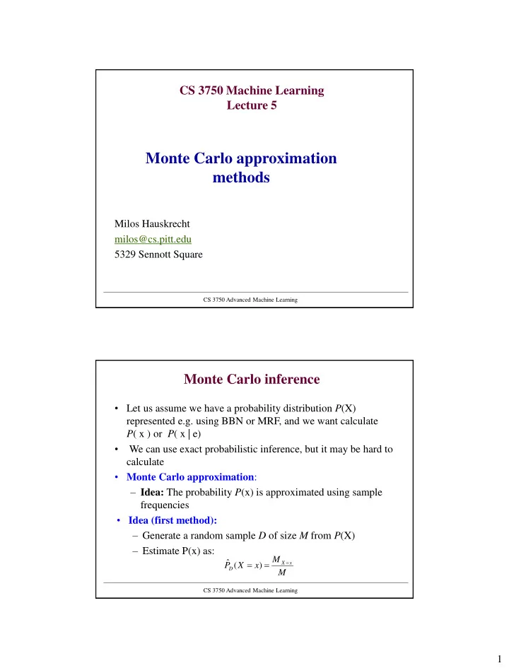
CS 3750 Machine Learning Lecture 5 Monte Carlo approximation methods Milos Hauskrecht milos@cs.pitt.edu 5329 Sennott Square CS 3750 Advanced Machine Learning Monte Carlo inference • Let us assume we have a probability distribution P (X) represented e.g. using BBN or MRF, and we want calculate P ( x ) or P ( x | e) • We can use exact probabilistic inference, but it may be hard to calculate • Monte Carlo approximation : – Idea: The probability P (x) is approximated using sample frequencies • Idea (first method): – Generate a random sample D of size M from P (X) – Estimate P(x) as: M ˆ ) X x P ( X x D M CS 3750 Advanced Machine Learning 1
Absolute Error Bound • Hoeffding’s bound lets us bound the probability with ˆ ( x ) which the estimate differs from by more ( ) P P x D than ˆ 2 2 M ( ( ) [ ( ) , ( ) ]) 2 P P x P x P x e D The bound can be used to decide on how many samples are required to achieve a desired accuracy: ln( 2 / ) M 2 2 3 Relative Error Bound • Chernoff’s bound lets us bound the probability of the estimate ˆ ( x ) ( ) P P x exceeding a relative error of the true value . D ˆ 2 ( ) / 3 MP x ( ( ) ( )( 1 )) 2 P P x P x e D • This leads to the following sample complexity bound: ln( 2 / ) M 3 2 ( ) P x 4 2
Monte Carlo inference challenges Challenge 1: How to generate M (unbiased) examples from the target distribution P(X) or P(X |e)? – Generating (unbiased) examples from P(X) or P(X|e) may be hard, or very inefficient Example: • Assume I have a distribution over 100 binary variables – There are 2 100 possible configurations of variable values • Trivial sampling solution: – Calculate and store the probability of each configuration – Pick randomly a configuration based on its probability • Problem: terribly inefficient in time and memory CS 3750 Advanced Machine Learning Monte Carlo inference challenges Challenge 2: How to estimate the expected value of f(x) for P(x) : • Generally, we can estimate this expectation by generating samples x[1], …, x[M] from P, and then estimating it as: [ ] ( ) ( ) E f p x f x dx [ ] ( ) ( ) E f P x f x P P x x 1 M ˆ ˆ [ ] ( [ ]) E f f x m P M m 1 0 2 ˆ • Using the central limit theorem, the estimate follows , N M – Where the variance for f(x) is 2 2 ( )[ ( ) ( ( ))] p x f x E f x dx P x • Problem: we are unable to efficiently sample P (x). What to do? CS 3750 Advanced Machine Learning 3
Central limit theorem • Central limit theorem: , , Let random variables form a random sample X X X 1 2 m 2 from a distribution with mean and variance , then if the sample n is large, the distribution m 1 m i m 2 or 2 ( , ) X N ( , / m ) X N m i m i 1 i 1 Effect of increasing the sample size m on the sample mean: 2 1.8 1.6 0 m 100 1.4 2 1.2 4 50 1 m 0.8 30 0.6 m 0.4 0.2 0 -2 -1.5 -1 -0.5 0 0.5 1 1.5 2 CS 3750 Advanced Machine Learning Monte Carlo inference: BBNs Challenge 1: How to generate M (unbiased) examples from the target distribution P(X) defined by a BBN? • Good news: Sample generation for the full joint defined by the BBN is easy – One top down sweep through the network lets us generate one example according to P(X) – Example: B E Examples are generated in a top down manner, A following the links M J CS 3750 Advanced Machine Learning 4
BBN sampling example P (B) P (E) T F T F Burglary 0.001 0.999 Earthquake 0.002 0.998 P (A|B,E) B E T F T T 0.95 0.05 T F 0.94 0.06 Alarm F T 0.29 0.71 F F 0.001 0.999 P (J|A) P (M|A) A T F A T F T 0.90 0.1 JohnCalls MaryCalls T 0.7 0.3 F 0.05 0.95 F 0.01 0.99 CS 3750 Advanced Machine Learning BBN sampling example P (B) P (E) T F T F Burglary 0.001 0.999 Earthquake 0.002 0.998 P (A|B,E) F B E T F T T 0.95 0.05 T F 0.94 0.06 Alarm F T 0.29 0.71 F F 0.001 0.999 P (J|A) P (M|A) A T F A T F T 0.90 0.1 JohnCalls MaryCalls T 0.7 0.3 F 0.05 0.95 F 0.01 0.99 CS 3750 Advanced Machine Learning 5
BBN sampling example P (B) P (E) T F T F Burglary 0.001 0.999 Earthquake 0.002 0.998 F P (A|B,E) F B E T F T T 0.95 0.05 T F 0.94 0.06 Alarm F T 0.29 0.71 F F 0.001 0.999 P (J|A) P (M|A) A T F A T F T 0.90 0.1 JohnCalls MaryCalls T 0.7 0.3 F 0.05 0.95 F 0.01 0.99 CS 3750 Advanced Machine Learning BBN sampling example P (B) P (E) T F T F Burglary 0.001 0.999 Earthquake 0.002 0.998 P (A|B,E) F F B E T F T T 0.95 0.05 T F 0.94 0.06 F Alarm F T 0.29 0.71 F F 0.001 0.999 P (J|A) P (M|A) A T F A T F T 0.90 0.1 JohnCalls MaryCalls T 0.7 0.3 F 0.05 0.95 F 0.01 0.99 CS 3750 Advanced Machine Learning 6
BBN sampling example P (B) P (E) T F T F Burglary 0.001 0.999 Earthquake 0.002 0.998 F P (A|B,E) F B E T F T T 0.95 0.05 T F 0.94 0.06 F Alarm F T 0.29 0.71 F F 0.001 0.999 P (J|A) P (M|A) A T F A T F T 0.90 0.1 JohnCalls MaryCalls T 0.7 0.3 F 0.05 0.95 F 0.01 0.99 F CS 3750 Advanced Machine Learning BBN sampling example P (B) P (E) T F T F Burglary 0.001 0.999 Earthquake 0.002 0.998 P (A|B,E) F F B E T F T T 0.95 0.05 T F 0.94 0.06 F Alarm F T 0.29 0.71 F F 0.001 0.999 P (J|A) P (M|A) A T F A T F T 0.90 0.1 JohnCalls MaryCalls T 0.7 0.3 F 0.05 0.95 F 0.01 0.99 F F CS 3750 Advanced Machine Learning 7
BBN sampling example P (B) P (E) T F T F Burglary 0.001 0.999 Earthquake 0.002 0.998 F P (A|B,E) F B E T F Sample: T T 0.95 0.05 T F 0.94 0.06 F F Alarm F F T 0.29 0.71 F F F 0.001 0.999 P (J|A) F F P(M|A) A T F A T F T 0.90 0.1 JohnCalls MaryCalls T 0.7 0.3 F 0.05 0.95 F 0.01 0.99 F F CS 3750 Advanced Machine Learning Monte Carlo inference: BBNs Challenge 1: How to generate M (unbiased) examples from the target distribution P(X) defined by BBN? • Good news: Sample generation for the full joint defined by the BBN is easy – One top down sweep through the network lets us generate one example according to P(X) – Example: B E Examples are generated in a top down manner, A following the links M J – Repeat many times to get enough of examples CS 3750 Advanced Machine Learning 8
Monte Carlo inference: BBNs Knowing how to generate efficiently examples from the full joint lets us efficiently estimate: – Joint probabilities over a subset variables – Marginals on variables • Example: B E A M J The probability is approximated using sample frequency # , samples with B T J T ~ N , B T J T ( , ) P B T J T N total # samples CS 3750 Advanced Machine Learning Monte Carlo inference: BBNs • MC approximation of conditional probabilities : – The probability can approximated using sample frequencies – Example: # , samples with B T J T ~ N , B T J T ( | ) P B T J T N J T # samples with J T • Solution 1 (rejection sampling): – Generate examples from P (X) which we know how to do efficiently • Use only samples that agree with the condition (J=T), the remaining samples are rejected • Problem: many examples are rejected. What if P (J=T) is very small? CS 3750 Advanced Machine Learning 9
Monte Carlo inference: BBNs • MC approximation of conditional probabilities • Solution 2 (likelihood weighting) – Avoids inefficiencies of rejection sampling – Idea: generate only samples consistent with an evidence (or conditioning event); If the value is set no sampling • Problem: using simple counts is not enough since these may occur with different probabilities • Likelihood weighting: – With every sample keep a weight with which it should count towards the estimate w B T ~ samples with B T and J T P ( B T | J T ) w B x samples with any value of B and J T CS 3750 Advanced Machine Learning BBN likelihood weighting example P (E) T F P (B) 0.002 0.998 T F Burglary 0.001 0.999 Earthquake E = F (set !!!) P (A|B,E) B E T F T T 0.95 0.05 T F 0.94 0.06 Alarm F T 0.29 0.71 F F 0.001 0.999 P (J|A) P (M|A) A T F A T F T 0.90 0.1 JohnCalls MaryCalls T 0.7 0.3 F 0.05 0.95 F 0.01 0.99 J = T (set !!!) CS 3750 Advanced Machine Learning 10
Recommend
More recommend
Explore More Topics
Stay informed with curated content and fresh updates.
