Model-based measurement of volatility using high-frequency data - PowerPoint PPT Presentation

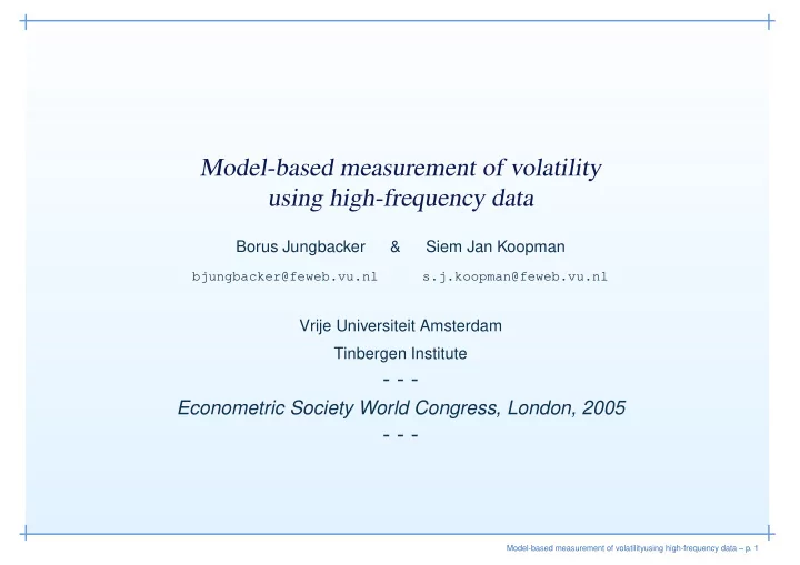
Model-based measurement of volatility using high-frequency data Borus Jungbacker & Siem Jan Koopman bjungbacker@feweb.vu.nl s.j.koopman@feweb.vu.nl Vrije Universiteit Amsterdam Tinbergen Institute - - - Econometric Society World Congress, London, 2005 - - - Model-based measurement of volatilityusing high-frequency data – p. 1

The paper in fast mode • Aim of the paper: to measure volatility within a model-based framework using high-frequency data; • Background: microstructure error exists in price data when observed at high-frequency; for measuring realised volatility, nonparametric methods have been considered to deal with microstructure error; • Problem: how to correct for microstructure error in a model-based framework for volatility ? • Solution: discretised pricing model can be represented as a dynamic latent process (random walk) with observation error; • Econometrics: how to estimate parameters from a non-linear state space model ? how to measure the latent volatility ? • Illustration: IBM tick-by-tick prices. Model-based measurement of volatilityusing high-frequency data – p. 2

Overview The contents of this presentation is • Introduction • Models for high-frequency prices • Estimation methods • Three months of IBM prices • Some more recent developments • Conclusion Model-based measurement of volatilityusing high-frequency data – p. 3

Introduction and notation The price of a financial asset is denoted by P t . Common assumption is that the log of P t can be represented by SDE d log P t = µ t ( ψ ) dt + σ t ( ψ ) dB t , t > 0 , (1) where µ t ( ψ ) is the drift (expected return), σ t ( ψ ) is a stochastic process (spot volatility), B t is standard Brownian motion and ψ is a vector of unknown parameters, see Campbell Lo and MacKinlay (1997) for more background. The variability in prices (integrated volatility) is � t σ ∗ 2 (0 , t ) = σ 2 t ( ψ ) dt. (2) 0 Actual volatility for interval [ t 1 , t 2 ] is σ ∗ 2 ( t 1 , t 2 ) = σ ∗ 2 (0 , t 2 ) − σ ∗ 2 (0 , t 1 ) . (3) Model-based measurement of volatilityusing high-frequency data – p. 4

Introduction and notation For the high-frequency data, we use notation as follows. • the observed log price at discrete time point t n (in seconds) is denoted by Y n = log P t n ; • number of time points (seconds) in trading day d is N d ; • time series Y 1 , Y 2 , . . . , Y N d (frequency in seconds) are log prices of trades on a particular day d . • value Y n is not available when no trade has taken place at time t n and is treated as missing; • number of trades is denoted by N ≤ N d so that we have N d − N missing values in day d . Model-based measurement of volatilityusing high-frequency data – p. 5

Realised volatility A natural estimator of actual volatility is realised volatility (RV) given by N d /m � ( Y mj − Y mj − m ) 2 , σ ∗ 2 ( t 0 , t N d ) = ˜ (4) j =2 where m is the sampling frequency. For example, when sampling frequency is 5 minutes, m equals 300 . In the case a transaction has not taken place at time n , so that Y n is missing in (4) , it can be approximated via interpolation methods, see Malliavin and Mancino (2002) and Hansen and Lunde (2004). An alternative semi-parametric approach for computing RV can be based on the estimated smoothness parameter for a trend (spline) model. Model-based measurement of volatilityusing high-frequency data – p. 6

Model for prices observed with micro-structure noise We consider model (1) : d log P t = µ t ( ψ ) dt + σ t ( ψ ) dB t , t > 0 , we assume that drift term equals zero: var ( P t + τ | P t ) only depends on the diffusion term σ t ( ψ ) . For volatility σ t ( ψ ) we consider various specifications. • First we take volatility as constant through time: σ t ( ψ ) = σ ( ψ ) ; • leads to following model for efficient price process, d log P t = σ ( ψ ) d B t , (5) where B t is standard Brownian motion. • trade prices Y n are observed with micro-structure noise U n ; Model-based measurement of volatilityusing high-frequency data – p. 7

Basic model for observed prices The discrete time model then becomes Y n = p n + σ U U n , U n ∼ IID (0 , 1) , (6) p n +1 = p n + σ ε ε n , ε n ∼ NID (0 , 1) , (7) where p n = log P t is unobserved price at time t = t n for n = 1 , . . . , N d ; • this leads to simple expression for actual volatility: σ ∗ 2 ( t n , t n +1 ) = ( t n +1 − t n ) σ 2 ε ; • it further implies that observed return R n = ∆ Y n +1 = ∆ p n +1 + σ U ∆ U n +1 = σ ε ε n + σ U U n +1 − σ U U n , follows R n ∼ MA (1) , see Harvey (1989). Model-based measurement of volatilityusing high-frequency data – p. 8

Basic model for observed prices For the discrete time model Y n = p n + σ U U n , U n ∼ IID (0 , 1) , p n +1 = p n + σ ε ε n , ε n ∼ NID (0 , 1) , assumption of constant volatility is too strong but it allows us to obtain a preliminary estimate of daily volatility. • standard Kalman filter methods can be used; • further it justifies (to some extent) the nonparametric estimates based on splines; Results based on this model will be presented later. Model-based measurement of volatilityusing high-frequency data – p. 9

Some considerations Aït Sahalia, Mykland and Zhang (2004) also consider local level model and observe that returns therefore follow an MA(1) process. they argue that distributional properties of U n do not matter asymptotically; “modelling the noise explicitly restores the first order statistical effect that sampling as often as possible is optimal” ; “this remains the case if one misspecifies the assumed distribution of the noise term” ; these quotes also endorse a modelling approach. They further discuss possible extensions: • the modelling of U n as a stationary autoregressive process; this can be easily done within the state space framework; • allowing for contemporaneous correlation between U n and ε n ; this correlation however is not identified in likelihood when both variances are unrestricted, see Harvey and Koopman (2000); it can be imposed nonetheless. Model-based measurement of volatilityusing high-frequency data – p. 10

Weight or Kernel functions for price extraction Weights are computed as in Koopman and Harvey (JEDC, 2003). (i) (ii) 0.15 q =0.3 and ρ = 0.2 q =0.3 and ρ = 0 0.10 0.10 0.05 0.05 −20 −10 0 10 20 −20 −10 0 10 20 (iii) (iv) 0.20 0.3 q =0.3 and ρ = 0.5 q =0.3 and ρ = 1 0.15 0.2 0.10 0.1 0.05 −20 −10 0 10 20 −20 −10 0 10 20 Model-based measurement of volatilityusing high-frequency data – p. 11

Intra-day seasonal patterns in volatility At the opening and closure of financial markets, price changes are more volatile than at other times during the trading session, see Dacorogna et al.(1993) and Andersen and Bollerslev (1997). Therefore we replace the spot volatility σ 2 in (5) by an intra-daily seasonal function t = σ 2 exp g ( t ) , t = log σ 2 + g ( t ) , σ 2 log σ 2 or where g ( t ) is deterministic (spline) function with diurnal pattern. The integrated volatility becomes � t � t σ ∗ 2 (0 , t ) = σ 2 s d s = σ 2 exp g ( s ) ds. (8) 0 0 Model-based measurement of volatilityusing high-frequency data – p. 12

Intra-day seasonal patterns in volatility Further we observe that • Actual volatility can be analytically derived or approximated by t n +1 � σ ∗ 2 ( t n , t n +1 ) ≈ σ 2 exp g ( s ) , s = t n with index step length very small. • The function g ( t ) = g ( t ; ψ ) depends on parameters collected in ψ together with the variances σ 2 ε and σ 2 U . • Standard time-varying Kalman filter methods can be used for maximum likelihood estimation of ψ and the measurement of actual volatility. Model-based measurement of volatilityusing high-frequency data – p. 13

Stochastic volatility To be more realistic, constant σ is replaced by stochastic process: d log P t = σ t d B (1) , t log σ 2 t = log σ ′ 2 t + ξ, (9) t d t + σ η d B (2) d log σ ′ 2 t = − λ log σ ′ 2 , t where B (1) and B (2) are independent Brownian motions while t t log σ ′ 2 t represents an Ornstein-Uhlenbeck process. Using the Euler-Maruyama method, a discrete representation is log P t n +1 = log P t n + σ n ε n , ε n ∼ NID (0 , 1) , log σ 2 n = log σ ′ 2 n + ξ, (10) log σ ′ 2 n +1 = (1 − λ ) log σ ′ 2 n + σ η η n , η n ∼ NID (0 , 1) . Note that λ = σ η = 0 implies constant volatility with log σ 2 n = ξ . Model-based measurement of volatilityusing high-frequency data – p. 14

Stochastic volatility • actual volatility is then approximated by � t n +1 σ ∗ 2 ( t n , t n +1 ) ≡ σ 2 s d s ≈ ( t n +1 − t n ) σ 2 n ; t n • model in terms of returns log( P t n +1 / P t n ) can also be considered; with micro-structure noise, the observed returns R n follow an MA (1) process; • with stochastic volatility, we obtain R n = σ n ε n + σ U W n , (11) where log σ 2 n is modelled as in (10) and W n = U n +1 − U n such that W n ∼ MA (1) ; • model (11) with σ U = 0 is the basic SV model. Model-based measurement of volatilityusing high-frequency data – p. 15