Model-Based Interpolation, Prediction, and Approximation - PDF document
Model-Based Interpolation, Prediction, and Approximation Statistical Computing for Uncertainty Analysis Antonio Possolo Statistical Engineering Division Information T echnology Laboratory August 4, 2011 1 / 28 Outline Statistical
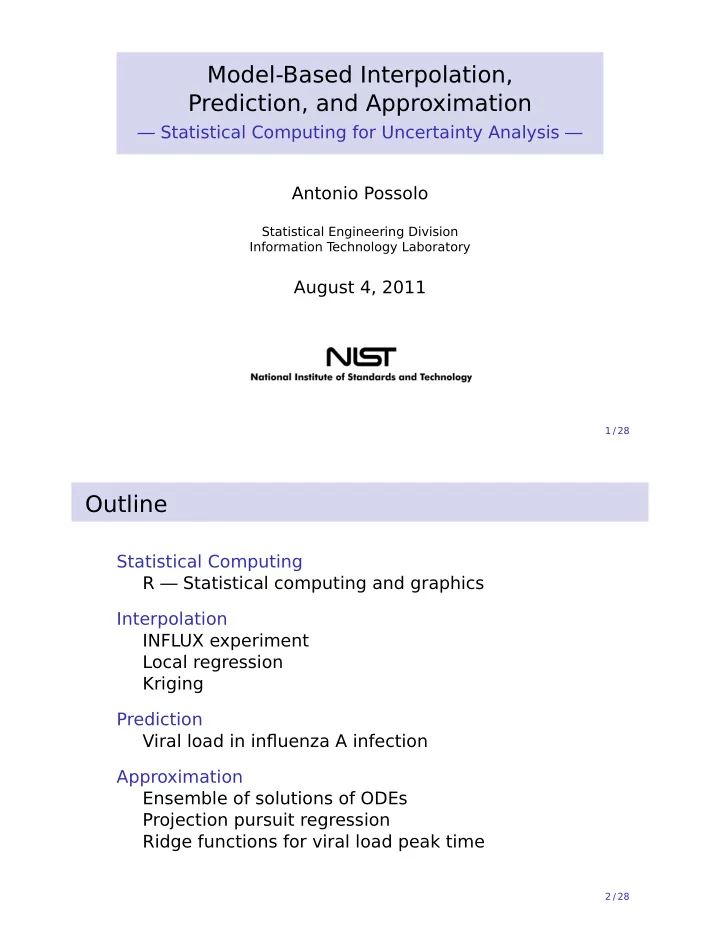
Model-Based Interpolation, Prediction, and Approximation — Statistical Computing for Uncertainty Analysis — Antonio Possolo Statistical Engineering Division Information T echnology Laboratory August 4, 2011 1 / 28 Outline Statistical Computing R — Statistical computing and graphics Interpolation INFLUX experiment Local regression Kriging Prediction Viral load in influenza A infection Approximation Ensemble of solutions of ODEs Projection pursuit regression Ridge functions for viral load peak time 2 / 28
R ◮ Programming environment for statistical computing, data analysis, and graphics ◮ www.r-project.org ◮ Free and open source ◮ Lingua franca of statistical computing: implementations of new statistical methods often first appear as R functions ◮ Ideal environment for uncertainty analysis, also well suited for prototyping general purpose scientific computing algorithms 3 / 28 INFLUX Experiment (Indianapolis, IN) — FLIGHT PATH 4 / 28
INFLUX Experiment — CO 2 measurements on curtain flight 5 / 28 Interpolation — PROBLEM ◮ Given Measured values y 1 , . . . , y m of real-valued function θ at 1 , . . . , m in metric space X ◮ Estimate θ ( ) for any “in the middle” of the { } ◮ Characterize uncertainty ( y ) associated with estimate 6 / 28
Model Based Interpolation — APPROACHES ◮ Model observations probabilistically — interpolation problem becomes statistical estimation problem y = θ ( ) + ε ◮ { ε } realized values of non-observable random variables (measurement errors) ◮ Interpolate signal, not signal + noise Local regression vs. Kriging ◮ θ locally quadratic ◮ θ realized value of Gaussian random function Θ 7 / 28 Local Regression 9.0 Signal ● Data = Signal + Noise ● ◮ Approximate θ locally by ● Local Regression ● 8.5 parabola at each target location ● 8.0 ◮ Fit each parabola by ● ● (robust) weighted least ● ● ● squares 7.5 ● ● ● ● ● Weights decrease to ● ● zero with increasing 7.0 ● distance to target ● ● ● location 0 5 10 15 20 25 8 / 28
Ordinary Kriging 9.0 Signal ● Data = Signal + Noise ● ◮ {Θ ( ) } Gaussian RVs ● Local Regression ● 8.5 with mean μ and Kriging covariance function ● γ ( h ) = Cov ( Θ ( ) , Θ ( + h )) 8.0 ● ● ● ● ◮ � θ ( ) is weighted ● 7.5 ● ● average of data { y } ● ● ● ● ● Weights depend on 7.0 ● γ ( h ) and on ● ● ● variances of { ε } 0 5 10 15 20 25 9 / 28 Kriging Assessment of Uncertainty ◮ Kriging often heralded as providing assessments of uncertainty of interpolations automatically ◮ In many instances of application, kriging’s built-in assessments underestimate uncertainty because one pretends that � γ = γ Bayesian kriging provides means to account for this often neglected component of uncertainty 10 / 28
Recommend
More recommend
Explore More Topics
Stay informed with curated content and fresh updates.
