Mode Estimation of Probabilistic Hybrid Systems Michael Hofbaur - PowerPoint PPT Presentation
Mode Estimation of Probabilistic Hybrid Systems Michael Hofbaur 1&2 & Brian C. Williams 1 1) Artificial Intelligence & Space Systems Laboratories MIT, USA 2) Department of Automatic Control, TU-Graz, Austria Motivation Advanced Life
Mode Estimation of Probabilistic Hybrid Systems Michael Hofbaur 1&2 & Brian C. Williams 1 1) Artificial Intelligence & Space Systems Laboratories MIT, USA 2) Department of Automatic Control, TU-Graz, Austria
Motivation Advanced Life Support System - BIO-Plex • Highly complex artifact • Long autonomous operation in a harsh environment • Robust operation – fault tolerance Monitoring and diagnosis capabilities are critical for building highly autonomous artifacts that can operate robustly in harsh environments of a long period of time. 2
Overview • Probabilistic Hybrid Automata – Model & Execution • Concurrent Probabilistic Hybrid Automata • Hybrid Estimation – Overview – intuitively & filtering background – Problem Formulation – A* Formulation • Example • Discussion & Conclusion 3
why Hybrid Mode/State Estimation? Monitoring and Diagnosis has to track the system’s behavior along both its continuous state changes and its discrete mode changes and their system-wide interaction. • operational modes 1200 crew requests entry to plant growth chamber 1100 CO 2 c oncent ration (p pm) 1000 • failure modes 900 800 crew enters chamber crew leaves 700 chamber • estimation and filtering of lighting fault 600 continuously valued 500 variables 400 600 700 800 900 1000 1100 1200 1300 1400 time (minutes) 4
Hybrid Model concurrent Probabilistic Hybrid Automata (cPHA) t r1 t r3 t c7 m c6 t c10 m r1 m r2 m r3 t r2 t r4 t c8 m c1 m c7 t c9 t c1 m r4 m r5 m r6 t c6 servo valve t c5 m c4 m c5 t l1 t c2 t c3 A concurrent Probabilistic Hybrid m c8 m c2 t c4 m c3 m l1 m l2 t l2 Automata (cPHA) is a hidden chamber control ... m l3 m l4 Markov model, encoded as a set of hybrid model gas sensor components with modes that exhibit a continuously valued dynamical behavior that is expressed by difference / algebraic equations. 5
Probabilistic Hybrid Automata x w , , F T X , , , U , T Probabilistic Hybrid Automata d d s � x x x d mode (discrete state) with domain X d ...{ x } ........ d c n � x c continuous state with domain � � w u u y ... ... u d discrete command with domain U d d c c m � u c continuous command with domain i m y c continuous output with domain � o F ................. discrete-time dynamics for each mode (sampling-period T s ) T ................. guarded probabilistic transitions between modes t r1 t r3 m r1 m r2 m r3 t r2 t r4 m r4 m r5 m r6 servo valve 6
Mode / State Transition Discrete mode changes and continuously valued evolution of the state variables take place at two different rates: a) continuous evolution is captured at the sampling-rate � � � � x f x , u , ' x , y g ( x , u , x ), c k ,( ) c k ,( 1) c k ,( 1) d ,( k 1) c k ,( ) c k ,( ) c k ,( ) d ,( ) k � � � � � t t T ( ) k ( k 1) s � b) probabilistic mode changes take place instantly ( x , u ) guard ������ � x x x , c ,( ) k d ,( ) k x ' , ' d ,( ) k c k ,( ) d ,( ) k c k ,( ) P t11 m 2 C 11 m 1 m 3 P t12 7
Mode / State Transition Mode Transition State Transition t (k) t’ (k) t (k+1) x ' x x d ,( ) k d ,( k 1) d ,( ) k � T i F j x ' x x ,( ) c k ,( ) c k ,( 1) c k � Mode transition : time proceeds only infinitesimally t’ (k) = t (k) + ε so that the evolution of the continuous state x c,(k) → x ’ c,(k) can be neglected: x ’ c,(k) = x c,(k) State transition : no transition is triggered ( x’ d,(k) = x d,(k+1) ) and time proceeds for one sampling period: t (k+1) = t (k) + T s . . The evolution of the continuous state x ’ c,(k) → x c,(k+1) is captured by the discrete-time dynamic model that holds for x’ d,(k) . 8
concurrent Probabilistic Hybrid Automata PHA component internal variable PHA4 PHA1 PHA2 continuous output / observed input u ci PHA3 variable y ci (cont.) discrete input u dj • concurrent PHA components are connected to inputs (continuous and discrete) and outputs of the cPHA and interconnected by internal variables. • observed variables = internal variable + additive Gaussian noise 9
Probabilistic Hybrid Automata , , u y v v , , , , A N N Concurrent Probabilistic Hybrid Automata c s o x y A ................ set of PHAs � u u u ... ... continuous and discrete command variables d c y c ................. observed continuous variables v s , v o ............ state disturbances and sensor noise inputs characterized by N x , N y � � � � x x x ... x c c 1 c 2 cl � x { , ,..., } x x x d d 1 d 2 dl PHA4 PHA1 PHA2 � � � � x f x , u , ' x v c k ,( ) c k ,( 1) c k ,( 1) d ,( k 1) s k ,( 1) PHA3 � � � � � � y g ( x , u , x ) v ( ) k c k ,( ) c k ,( ) d ,( ) k o k ,( ) 10
Roadmap • Probabilistic Hybrid Automata – Model & Execution • Concurrent Probabilistic Hybrid Automata • Hybrid Estimation – Overview – intuitively & filtering background – Problem Formulation – A* Formulation • Example • Discussion & Conclusion 11
Hybrid Mode / State Estimation Task Overview: PHA4 PHA1 PHA2 continuous PHA3 output / observed input u ci variable y ci (cont.) discrete input u cj Hybrid Estimation Problem: Given a cPHA model for a system, a sequence of observations and the history of the control inputs generate the leading set of most likely states at time-step k 12
Background: Multi-Model Estimation sensor signals y c estimated mode & state { x d , x c } Hypothesis and control inputs u c Selection Continuous Estimators and (e.g. Kalman Filter Bank) Data Fusion State Estimator : Static filter bank Hypothesis selection and Data Fusion: that maintains a trajectory estimate for determines the most likely mode and every mode. continuous state for the system as well as provides the initialization for the filter bank. advantages: high fidelity estimation of continuous behaviors noise handling and incipient fault detection disadvantages: limited to tracking a small number of hypothesis (limited size of the filter bank) 13
hybrid Mode / State Estimation estimated mode & state x = { x d , x c } Concurrent PHA Model Hybrid and it’s belief state h [ x ] sensor signals y c and Mode control inputs u c , u d Continuous Estimators Estimator (e.g. Kalman Filter Bank) Hybrid State Estimator Hybrid Mode estimator: Maintains the set of most likely hybrid Determines for each trajectory the possible state estimates as a set of trajectories. transitions, and specifies (dynamically) the A Hidden Markov Model style belief candidate trajectories to be tracked by the state update is used to determine the continuous state estimators. likelihood for each traced trajectory 14
hybrid Mode/State Estimation At each time step k , we evaluate for each trajectory: old estimate: x (k-1) = { x d,(k-1) , x c,(k-1) } , h (k-1) 15
hybrid Mode Estimation At each time step k , we evaluate for each trajectory: old estimate: x ’ (k-1) = { x ’ d,(k-1) , x c,(k-1) } , x (k-1) = { x d,(k-1) , x c,(k-1) } , h (k-1) h’ = P t h (k-1) P t mode transition: x d,(k-1) = m i → x ’ d,(k-1) = m j 16
Transition Probability P o m 3 P t13 P t11 C 12 C 11 m 1 probability P C of guard C 12 P t12 P t14 m 2 m 4 C 12 guards the transition to either m 3 ( nominal transition) c CO2 580 or to m 4 ( failure transition): mean of estimated CO 2 guard boundary concentration � C : c 580 ppm 12 CO 2 transition probability = guard probability * thread probability 17
hybrid Mode Estimation At each time step k , we evaluate for each trajectory: new estimate old estimate: x ’ (k-1) = { x ’ d,(k-1) , x c,(k-1) } , x (k) = { x d,(k) , x c,(k) } , x (k-1) = { x d,(k-1) , x c,(k-1) } , h (k-1) h’ = P t h (k-1) h (k) = P o h’ P o P t continuous behavior mode transition: x d,(k-1) = m i → x ’ d,(k-1) = m j x ’ c,(k-1) → x c,(k) , x d,(k) = x ’ d,(k-1) 18
Observation Probability P t We compare the sensor signal y c(k) with its estimation for mode m j using an extended Kalman filter. operation performed by an (extended) Kalman filter: x c,(k-1) , P (k-1) , u c,(k-1) → • state prediction: x ’ c,(k) , P ’ (k) → • residual calculation: x ’ c,(k) , P ’ (k) , y c(k) r (k) , S (k) , P o → • Kalman filter gain calculation: P ’ (k) k (k) x ’ c,(k) , P ’ (k) , k (k) , r (k) → x c,(k) , P (k) • state estimate refinement: − − = T 1 r S r P e o → one extended Kalman filter for each hypothesis 19
exponential Explosion At each time step k , we evaluate for each trajectory: new estimate old estimate: x ’ (k-1) = { x ’ d,(k-1) , x c,(k-1) } , x (k) = { x d,(k) , x c,(k) } , x (k-1) = { x d,(k-1) , x c,(k-1) } , h (k-1) h’ = P t h (k-1) h (k) = P o h’ P o continuous behavior mode transition: x d,(k-1) = m i → x ’ d,(k-1) = m j x ’ c,(k-1) → x c,(k) , x d,(k) = x ’ d,(k-1) The number of possible transitions at each time step can be very large: E.g. a model with 10 components, each of which can transition to 3 successor modes has 3 10 = 59049 possible successor modes for each trajectory at each time step ! 20
Recommend
More recommend
Explore More Topics
Stay informed with curated content and fresh updates.
