Methods for calculating rare event dynamics and pathways of - PowerPoint PPT Presentation
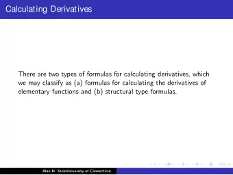
Methods for calculating rare event dynamics and pathways of solid-solid phase transitions Graeme Henkelman University of Texas at Austin -dynamics Solid-state nudged elastic band rock 4.06 4.06 salt wurtzite 4.38 4.38 Classes
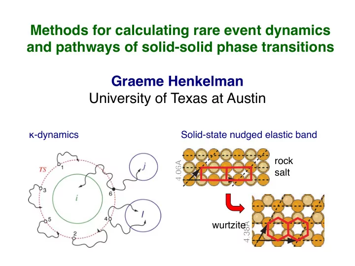
Methods for calculating rare event dynamics and pathways of solid-solid phase transitions Graeme Henkelman University of Texas at Austin κ -dynamics Solid-state nudged elastic band rock 4.06Å 4.06Å salt wurtzite 4.38Å 4.38Å
Classes of Dynamical Systems Energy Landscape: Smooth Rough Final State: Initial Final Final Known Initial Unknown ? Initial
Transition state theory A statistical theory for calculating the rate of slow thermal processes -- rare event dynamics Requires an N-1 dimensional dividing surface x = x † that is a bottleneck for the transition: P k TST = 1 δ ( x − x † ) | v ⊥ | ⌦ ↵ R 2 R Harmonic transition state theory Find saddle points on the energy surface Rate of escape through each saddle point region: Q N ✓ ◆ − ∆ E i =1 ν i k HTST = exp Q N − 1 j =1 ν † k B T ∆ E j
KMC: the Good, the Bad, and the Ugly The Good For rare event systems where transition rates are defined by first-order rate constants, KMC is an exact stochastic solution to the kinetic master equation. where where μ is random on (0,1] The Bad It is very hard to determine all possible kinetic events available to the simulation. It is very hard to calculate an exact rate for a process, let alone all of them. Typically limited to transition state theory (e.g. harmonic TST within aKMC). The Ugly It’s a lot of work calculating all possible events and rates to find one trajectory.
Dynamical corrections to TST TST assumes that all trajectories that violation cross the TS are reactive trajectories. of TST Dynamical correction factor : the ratio of successful trajectories to number of crossing points ratio between the TST and true rate: both total escape rate and by product: A successful trajectory: Example: 1) trajectory must go directly to products without recrossing the TS 2) trajectory must start in initial state
The κ -dynamics algorithm 1. Choose a reaction coordinate and sample a transition state (TS) surface 2. Launch short time trajectories until one goes directly to a product and starts in the initial state; record the number, N 3. If no successful trajectory within N max , push TS up in free energy and go to 2 4. Calculate k TST for successful TS surface (parallel tempering, WHAM) 7 5. Update the simulation clock by 2 6 1 3 4 5 where μ n are random numbers on (0,1] 6. Repeat procedure in product state C.-Y. Lu, D. E. Makarov, and G. Henkelman, J. Chem. Phys. 133 , 201101 (2010).
Sketch of proof that κ -dynamics is exact (1) Branching ratio where The probability of reaching state j is: sampled A. Voter and J. D. Doll JCP 82, 1 (1985) (2) Reaction time What we want: where is the true rate What we have where in κ -dynamics: (1 success)(N-1 failures) Connection with TST rate: Erlang N-distribution Combining: the correct distribution based upon the true rate
Reaction coordinate test Bond stretching parameter Bond-boost : specifies the stretch in the most-stretched bond: R. A. Miron and K. A. Fichthorn, JCP 119, 6210 (2003) Al/Al(100), hop on frozen surface Exchange on relaxed surface κ -dynamics k TST TST+ κ hTST κ -dyn κ -dynamics rates are correct and independent of reaction coordinate
Branching ratio test Comparison of reaction products for classical dynamics and κ -dynamics Al/Al(100), relaxed surface 1.0 � direct MD Branching ratio ��� κ-dynamics harmonic TST �� �� 0.5 �� �� � � � � � � � � 200K 400K 0.0 1 2 3 4 5 6 7 8 1 2 3 4 5 6 7 8 Reaction mechanism
κ -dynamics trajectories Al/Al(100) island ripening Al/Al(100) pyramid collapse
zite Solid-solid phase transitions Some transitions involve both change in atomic and cell degrees of freedom E.g. CdSe: 4.06Å 4.06Å 4.38Å 4.38Å rock salt wurtzite Potential parameters: E. Rabani, J. Chem. Phys. 116 , 258 (2002).
zite Nudged Elastic Band Method Pioneering work i − 1 Pratt, Elber, Karplus, ... and others F i Initial i ˆ F τ i i Nudged elastic band NEB F F S i i Images connect initial and final states i + 1 NEB force on each image: NEB MEP Perpendicular component (potential): Final Parallel component (springs): [1] H. Jónsson, G. Mills, and K.W. Jacobsen, in Classical and Quantum Dynamics in Condensed Phase Simulations , 385 (1998). [2] G. Henkelman and H. Jónsson, J. Chem. Phys. 113 , 9978 (2000). [3] G. Henkelman, B. P. Uberuaga, and H. Jónsson, J. Chem. Phys. 113 , 9901 (2000).
Danger of assuming a reaction coordinate The x-coordinate separates initial from final state, but is not a suitable reaction coordinate: A drag calculation along x (black points) misses Initial initial the saddle point where 3 drag direction the reaction coordinate NEB follows the y -direction saddle r AB y The resulting barrier is 2 reaction i n under-estimated: i t coordinate i a l b a n d NEB initial 1 energy drag drag final Final final reaction coordinate -2 -1 0 1 x x
Cell variables vs atomic coordinates Two pathways for the same solid-solid phase transition in CdSe a) atom dominated b) cell dominated atom dominated cell dominated NEB calculations in only atomic [1] or cell (RNM) initial [2] coordinates have the (rock salt) 4.06 Å 4.06Å 4.06Å 4.06Å errors found in drag methods. Requires a 9.08 Å 11.49 Å unified approach transition state 4.22 Å 4.20Å 4.20Å 4.20Å 3 initial drag direction NEB 9.36 Å 10.98 Å saddle r AB cell 2 initial band final (wurtzite) 1 4.38 Å 4.38Å 4.38Å 4.38Å drag final 8.75 Å 8.75 Å -2 -1 0 1 x atoms [1] D. R. Trinkle, R. G. Hennig, S. G. Srinivasan, et al., PRL 91 , 025701 (2003). [2] K. J. Caspersen and E. A. Carter, PNAS 102 , 6738 (2005).
Choice of cell representation Cell coordinates Choose a representation which does not allow for v 3 = (h ,h ,h ) 3x 3y 3z net rotation of the lattice v 2 = (h ,h ,0) 2x 2y v 1 = (h ,0,0) 1x Changes in the cell are represented as strain periodic solid expanded periodic solid Strain describes changes in the lattice which is ( ) δ 0 ɛ = 0 δ invariant to the unit cell
Combining atomic and cell variables (G-SSNEB) Single displacement vector: change in cell shape change in atom positions Jacobian to combine different units Requirement : reaction pathways should be independent of unit cell size and shape -- the path should be a property of the infinite solid Unit of length, average distance between atoms: volume Scaling of atomic displacements with size: Choose J so that J ε has same units and scaling as Δ R : Similar logic applies to the stress / force vector:
Results initial state initial state saddle 16 meV saddle 20 20 15 meV energy / atom (meV) energy / atom (meV) 13 meV 12 meV 0 0 G-SSNEB RNM G-SSNEB RNM -20 -20 final state final state -40 -40 NEB NEB -60 -60 initial final initial final G-SSNEB G-SSNEB saddle saddle RNM NEB NEB RNM Atom-dominated process: Cell-dominated process: RNM fails; NEB / G-SSNEB work NEB fails; RNM / G-SSNEB work
Scaling with system size Minimum energy path is insensitive to unit cell size and shape: atoms / cell 20 8 32 energy / atom (meV) 0 72 128 128 -20 transition state -40 -60 -2 -1 0 1 distance / � N (Å)
Change of mechanism With increasing system size: The mechanism changes from a concerted bulk process (cell dominated) to a local (atom dominated) b 2d (line defect) a 3d (bulk concerted) 1d (point defect) 10 c energy (eV) b 1 a a 0.1 10 100 1,000 10,000 number of atoms in unit cell
Movies Concerted mechanism Local mechanism
Local process in detail Complex mechanism: a 2 a 0 energy / atom (meV) 1 c -20 b -40 0 -60 -80 initial final c b
Research Group Penghao Xiao Chun-Yaung (Albert) Lu Daniel Sheppard
Acknowledgments Funding Research Group and Collaborators DOE - EFRC, SISGR Chun Yaung Lu (graduate student, now at LANL) NSF - CAREER, NIRT Daniel Sheppard (graduate student, now at LANL) Welch Foundation Penghao Xiao (graduate student) AFOSR Rye Terrell (graduate student) Sam Chill (graduate student) Computer Time Will Chemelewski (graduate student) Texas Advanced Computing Center Dmitrii Makarov (U. Texas, Austin) EMSL at PNNL Hannes Jónsson (U. Iceland) CNM at ANL Andreas Pederson (U. Iceland) Duane Johnson (Iowa State/Ames Lab) Software tools http://theory.cm.utexas.edu/vtsttools/ � AKMC , Dimer, (SS)NEB , and dynamical matrix � methods implemented in the VASP code http://theory.cm.utexas.edu/bader/ � Bader charge density analysis http://theochem.org/EON/ � The EON project for long time scale simulations http://theory.cm.utexas.edu/code/tsase/ � Transition state simulation environment (for ASE)
Recommend


More recommend
Explore More Topics
Stay informed with curated content and fresh updates.