Calculating distributions Chung-chieh Shan Indiana University - PowerPoint PPT Presentation
Calculating distributions Chung-chieh Shan Indiana University 2018-09-21 Calculating distributions executable meaningful Calculating distributions executable meaningful Id also like to address this concept of being fake or
Calculating distributions Chung-chieh Shan Indiana University 2018-09-21
Calculating distributions executable meaningful
Calculating distributions executable meaningful
‘ I’d also like to address this concept of being “fake” or “calculating. ” If being “fake” means not thinking or feeling the same way in one moment than you thought or felt in a different moment, then lord help us all. If being “calculating” is thinking through your words and actions and modeling the behavior you would like to see in the world, even when it is difficult, ’ then I hope more of you will become calculating. —BenDeLaCreme
Creative definitions and reasoning from first principles Symbolic representations of common definition patterns Mechanical operations for common reasoning patterns Virtuous cycle of automation and exploration (Buchberger)
Creative definitions natural and reasoning from first numbers principles Symbolic representations unary, of common definition binary patterns Mechanical operations < , + , ÷ for common reasoning patterns Virtuous cycle rationals, of automation reals, and exploration polynomials (Buchberger)
Creative definitions natural probability and reasoning from first numbers distributions principles Symbolic representations unary, table, of common definition binary Bayes net, patterns probabilistic program Mechanical operations < , + , ÷ recognize, for common reasoning integrate, patterns disintegrate Virtuous cycle rationals, inference, of automation reals, learning, and exploration polynomials optimization (Buchberger)
An unknown random process yields a We flip the coin 3 times and observe THH. stateless coin that can be flipped repeatedly What is the probability that the next flip to produce heads (H) or tails (T). produces H versus T? We assume that the probability p that the (adapted from Eddy) coin produces H each time is distributed uniformly between 0 and 1 by the process. 8
bind disintegrate bind integrate Pr( p ,� Pr( p | � Pr( p , y | � Pr( y | � Pr( p ) x ) x ) x ) x ) An unknown random process yields a We flip the coin 3 times and observe THH. stateless coin that can be flipped repeatedly What is the probability that the next flip to produce heads (H) or tails (T). produces H versus T? We assume that the probability p that the (adapted from Eddy) coin produces H each time is distributed uniformly between 0 and 1 by the process. 9
bind disintegrate bind integrate Pr( p ,� Pr( p | � Pr( p , y | � Pr( y | � Pr( p ) x ) x ) x ) x ) p p p p p y y � x � � � x x x 10
bind disintegrate bind integrate Pr( p ,� Pr( p | � Pr( p , y | � Pr( y | � Pr( p ) x ) x ) x ) x ) p p p p p y y � x � � � x x x 11
bind disintegrate bind integrate Pr( p ,� Pr( p | � Pr( p , y | � Pr( y | � Pr( p ) x ) x ) x ) x ) p p p p p y y � x � � � x x x 12
bind disintegrate bind integrate Pr( p ,� Pr( p | � Pr( p , y | � Pr( y | � Pr( p ) x ) x ) x ) x ) p p p p p y y � x � � � x x x 13
bind disintegrate bind integrate Pr( p ,� Pr( p | � Pr( p , y | � Pr( y | � Pr( p ) x ) x ) x ) x ) p p p p p y y � x � � � x x x 14
bind disintegrate bind integrate Pr( p ,� Pr( p | � Pr( p , y | � Pr( y | � Pr( p ) x ) x ) x ) x ) p p p p p y y � x � � � x x x = = = 15
bind disintegrate bind integrate Pr( p ,� Pr( p | � Pr( p , y | � Pr( y | � Pr( p ) x ) x ) x ) x ) p p p p p y y � x � � � x x x simplify = = = p p y y 16
sampler prediction problems. A emerged Approximations calculated exactly 1. Introduction The hidden Markov model (HMM) (Rabiner, 1989) is one of the most widely used models in machine learn- ing and statistics for sequential or time series data. Infinite Hidden Markov Model The HMM consists of a hidden state sequence with 2. The Infinite Hidden Markov Model dynamics, and independent observations at We start this section by describing the finite HMM, There are state. then taking the infinite limit to obtain an intuition hyperparameters can will use this in the experiments to follo for the infinite HMM, followed by a more precise def- The in- inition. A finite HMM consists of a hidden state se- , s , . . . , s T ) and a corresponding ob- d- 3. The Gibbs Sampler The Gibbs sampler was the first sampling algorithm Each state um- . , y ). for the iHMM that converges to the true posterior. W not suffer from this One proposal builds on the direct assignment sampling the whole sequence s in one go. scheme for the HDP in (Teh et al., 2006) by marginal- hidden variables π , φ from (2), (3) and 4. The Beam Sampler The forward-backward algorithm does not apply to implicit in β . Thus we the iHMM because the number of states, and hence base data. curve shows the Gibbs line show the one standard deviation error the number of potential state trajectories, are infinite. The idea of beam sampling is to introduce auxiliary h that conditioned on u the number 5. Experiments We evaluate the beam sampler on two artificial and probability is finite. Now algorithm datasets to illustrate the following properties: infinite capacit mixes in much fewer iterations 17 exity per is
sampler prediction problems. A emerged Approximations calculated exactly 1. Introduction The hidden Markov model (HMM) (Rabiner, 1989) is one of the most widely used models in machine learn- ing and statistics for sequential or time series data. Infinite Hidden Markov Model � = The HMM consists of a hidden state sequence with ∈ � 2. The Infinite Hidden Markov Model ⊗ � t h T h a t e n µ a n dynamics, and independent observations at d T m u µ t u a a l r e l y m u s i n t u g a l u l a l y We start this section by describing the finite HMM, r a b There are o n s o t h l u t e e l c o m p l e state. a m e r e n t n o f then taking the infinite limit to obtain an intuition u l R l f , R c o r b o . T t h h e hyperparameters can will use this in the experiments to follo µ s a e t n d T µ for the infinite HMM, followed by a more precise def- . L e . The t T h µ e n a in- t h n d T e r µ e e x i R b e s t t h inition. A finite HMM consists of a hidden state se- s a e v e r s R i o n o f t h e d e n s i t , s , . . . , s T ) and a corresponding ob- y d- 3. The Gibbs Sampler The Gibbs sampler was the first sampling algorithm Each state µ � d x � um- r � d y x � � . , y ). y � R = for the iHMM that converges to the true posterior. W T not suffer from this µ One proposal builds on the direct assignment sampling � d the whole sequence s in one go. x � d y � R x scheme for the HDP in (Teh et al., 2006) by marginal- � y � < ∞ a n d r � x � y � hidden variables π , φ from (2), (3) and = 1 / r � y � x � f 4. The Beam Sampler o r a l l x � y The forward-backward algorithm does not apply to implicit in β . Thus we ∈ E d x � the iHMM because the number of states, and hence base d y � = µ � d x � d y data. s curve shows the Gibbs line show the one standard deviation error y m m the number of potential state trajectories, are infinite. e t r i c (i) f(x ) The idea of beam sampling is to introduce auxiliary h that conditioned on u the number 5. Experiments We evaluate the beam sampler on two artificial and probability is finite. Now (i+1) (i+1) u x algorithm datasets to illustrate the following properties: infinite capacit mixes in much fewer iterations 18 exity per is
bind disintegrate bind integrate Pr( p ,� Pr( p | � Pr( p , y | � Pr( y | � Pr( p ) x ) x ) x ) x ) 19
bind disintegrate bind integrate Pr( p ,� Pr( p | � Pr( p , y | � Pr( y | � Pr( p ) x ) x ) x ) x ) s i m p l i f y 400 Time in seconds 200 PSI 200 400 600 800 20 Data size
Recommend
More recommend
Explore More Topics
Stay informed with curated content and fresh updates.
