MDPs and Value Iteration 2/20/17 Recall: State Space Search - PowerPoint PPT Presentation

MDPs and Value Iteration 2/20/17

Recall: State Space Search Problems • A set of discrete states • A distinguished start state • A set of actions available to the agent in each state • An action function that, given a state and an action, returns a new state • A set of goal states , often specified as a function • A way to measure solution quality

What if actions aren’t perfect? • We might not know exactly which next state will result from an action. • We can model this as a probability distribution over next states.

Search with Non-Deterministic Actions • A set of discrete states • A distinguished start state • A set of actions available to the agent in each state • An action function that, given a state and an action, returns a new state a probability distribution over next states • A set of goal states , often specified as a function • A way to measure solution quality • A set of terminal states • A reward function that gives a utility for each state

Markov Decision Processes (MDPs) Named after the “Markov property”: if you know the state then you know the transition probabilities. • We still represent states and actions. • Actions no longer lead to a single next state. • Instead they lead to one of several possible states, determined randomly. • We’re now working with utilities instead of goals. • Expected utility works well for handling randomness. • We need to plan for unintended consequences. • Even an optimal agent may run forever!

State Space Search MDPs • States: S • States: S • Actions: A s • Actions: A s • Transition function • Transition probabilities • F(s, a) = s’ • P(s’ | s, a) • Start ∈ S • Start ∈ S • Goals ⊂ S • Terminal ⊂ S • Action Costs: C(a) • State Rewards: R(s) • Can also have costs: C(a)

We can’t rely on a single plan! Actions might not have the outcome we expect, so our plans need to include contingencies for states we could end up in. Instead of searching for a plan , we devise a policy . A policy is a function that maps states to actions. • For each state we could end up in, the policy tells us which action to take.

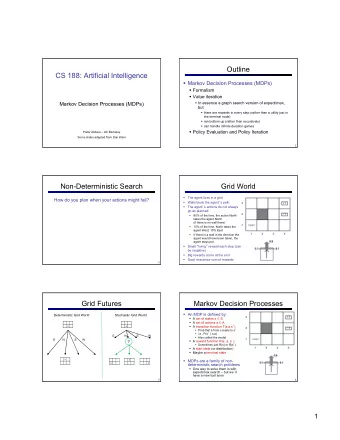
A simple example: Grid World end +1 end -1 start If actions were deterministic, we could solve this with state space search. • (3,2) would be a goal state • (3,1) would be a dead end

A simple example: Grid World end +1 end -1 start • Suppose instead that the move we try to make only works correctly 80% of the time. • 10% of the time, we go in each perpendicular direction, e.g. try to go right, go up instead. • If impossible, stay in place.

A simple example: Grid World end +1 end -1 start • Before, we had two equally-good alternatives. • Which path is better when actions are uncertain? • What should we do if we find ourselves in (2,1)?

Discount Factor Specifies how impatient the agent is. Key idea: reward now is better than reward later. • Rewards in the future are exponentially decayed. • Reward t steps in the future is discounted by 𝜹 t U = γ t · R t • Why do we need a discount factor?

Value of a State • To come up with an optimal policy, we start by determining a value for each state. • The value of a state is reward now, plus discounted future reward: V ( s ) = R ( s ) + γ [future value] • Assume we’ll do the best thing in the future.

Future Value • If we know the value of other states, we can calculate the expected value of each action: P ( s 0 | s, a ) · V ( s 0 ) X E ( s, a ) = s 0 • Future value is the expected value of the best action: max E ( s, a ) a

Value Iteration • The value of state s depends on the value of other states s’ . • The value of s’ may depend on the value of s . We can iteratively approximate the value using dynamic programming. • Initialize all values to the immediate rewards. • Update values based on the best next-state. • Repeat until convergence (values don’t change).

Value Iteration Pseudocode values = {state : R(state) for each state} until values don’t change: prev = copy of values for each state s: initialize best_EV for each action: EV = 0 for each next state ns: EV += prob * prev[ns] best_EV = max(EV, best_EV) values[s] = R(s) + gamma*best_EV

Value Iteration on Grid World V (2 , 2) = 0 + γ · max [ E ((2 , 2) , u ) , E ((2 , 2) , d ) , 0 0 0 +1 E ((2 , 2) , l ) , E ((2 , 2) , r ) ] 0 0 -1 V (2 , 1) = 0 + γ · max [ E ((2 , 1) , u ) , 0 0 0 0 E ((2 , 1) , d ) , E ((2 , 1) , l ) , E ((2 , 1) , r ) ] V (3 , 0) = 0 + γ · max [ E ((3 , 0) , u ) , E ((3 , 0) , d ) , discount =.9 E ((3 , 0) , l ) , E ((3 , 0) , r ) ]

Value Iteration on Grid World V (2 , 2) = γ · max[ . 8 · 0 + . 1 · 0 + . 1 · 1 , . 8 · 0 + . 1 · 1 + . 1 · 0 , 0 0 .72 +1 . 8 · 0 + . 1 · 0 + . 1 · 0 , . 8 · 1 + . 1 · 0 + . 1 · 0] 0 0 -1 V (2 , 1) = γ · max [ . 8 · 0 + . 1 · 0 + . 1 · − 1 , 0 0 0 0 . 8 · 0 + . 1 · − 1 + . 1 · 0 , . 8 · 0 + . 1 · 0 + . 1 · 0 , . 8 · − 1 + . 1 · 0 + . 1 · 0 ] V (3 , 0) = γ · max [ . 8 · − 1 + . 1 · 0 + . 1 · 0 , . 8 · 0 + . 1 · 0 + . 1 · 0 , . 8 · 0 + . 1 · 0 + . 1 · − 1 , discount =.9 . 8 · 0 + . 1 · − 1 + . 1 · 0 ]

Value Iteration on Grid World Exercise: Continue value iteration 0 .5184 .7848 +1 0 .4284 -1 0 0 0 0 discount =.9

What do we do with the values? When values have converged, the optimal policy is to select the action with the highest expected value at each state. +1 .64 .74 .85 -1 .57 .57 .49 .43 .48 .28 • What should we do if we find ourselves in (2,1)?