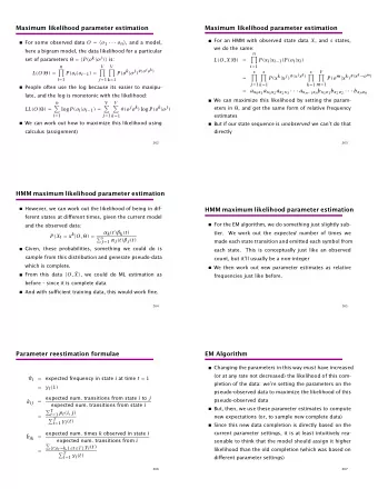
Maximum Likelihood Setting parameters Chris Williams, School of - PowerPoint PPT Presentation

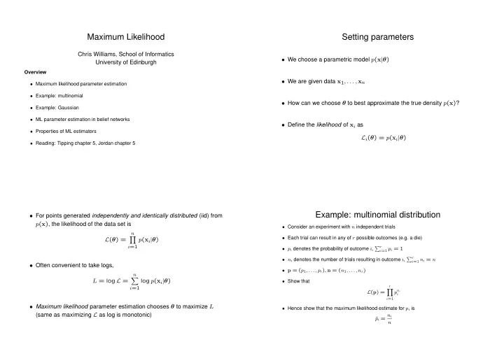
Maximum Likelihood Setting parameters Chris Williams, School of Informatics • We choose a parametric model p ( x | θ ) University of Edinburgh Overview • We are given data x 1 , . . . , x n • Maximum likelihood parameter estimation • Example: multinomial • How can we choose θ to best approximate the true density p ( x ) ? • Example: Gaussian • ML parameter estimation in belief networks • Define the likelihood of x i as • Properties of ML estimators L i ( θ ) = p ( x i | θ ) • Reading: Tipping chapter 5, Jordan chapter 5 Example: multinomial distribution • For points generated independently and identically distributed (iid) from p ( x ) , the likelihood of the data set is • Consider an experiment with n independent trials n • Each trial can result in any of r possible outcomes (e.g. a die) � L ( θ ) = p ( x i | θ ) i =1 • p i denotes the probability of outcome i , � r i =1 p i = 1 • n i denotes the number of trials resulting in outcome i , � r i =1 n i = n • Often convenient to take logs, • p = ( p 1 , . . . , p r ) , n = ( n 1 , . . . , n r ) n � L = log L = log p ( x i | θ ) • Show that r i =1 � p n i L ( p ) = i i =1 • Maximum likelihood parameter estimation chooses θ to maximize L • Hence show that the maximum likelihood estimate for p i is (same as maximizing L as log is monotonic) p i = n i ˆ n

Gaussian example • For the multivariate Gaussian n µ = 1 • likelihood for one data point x i in 1-d � ˆ x i � ( x i − µ ) 2 � n 1 p ( x i | µ, σ 2 ) = i =1 (2 πσ 2 ) 1 / 2 exp − 2 σ 2 n Σ = 1 µ ) T ˆ • Log likelihood for n data points � ( x i − ˆ µ )( x i − ˆ n n i =1 L = − 1 � log(2 πσ 2 ) + ( x i − µ ) 2 � � 2 σ 2 i =1 • Show that n µ = 1 � ˆ x i n i =1 • and n σ 2 = 1 � µ ) 2 ˆ ( x i − ˆ n i =1 ML parameter estimation in fully observable belief Example of ML Learning in a Belief Network networks R S H W k � n n n n P ( X 1 , . . . , X k | θ ) = P ( X j | Pa j , θ j ) j =1 n n n n y n y y • Show that parameter estimation for θ j depends only on statistics of ( X j , Pa j ) n n n n • Discrete variables: CPTs n n n n n jk P ( X 2 = s k | X 1 = s j ) = n n n y � l n jl n n n n Rain Sprinkler • Gaussian variables n n n y Y = µ y + w y ( X − µ x ) + N y n n n n Estimation of µ x , µ y , w y and v N y is a linear regression problem Watson Holmes y y y y

Properties of ML estimators From the table of data we obtain the following ML estimates for the CPTs • An estimator is consistent if it converges to the true value as the sample P ( R = yes ) = 2 / 10 = 0 . 2 size n → ∞ . Consistency is a “good thing” P ( S = yes ) = 1 / 10 = 0 . 1 P ( W = yes | R = yes ) = 2 / 2 = 1 • Bias P ( W = yes | R = no ) = 2 / 8 = 0 . 25 An estimator ˆ θ is unbiased if E [ˆ θ ] = θ . The expectation is wrt data drawn from the model p ( ·| θ ) P ( H = yes | R = yes, S = yes ) = 1 / 1 = 1 . 0 P ( H = yes | R = yes, S = no ) = 1 / 1 = 1 . 0 • The estimator ˆ µ for the mean of a Gaussian is unbiased P ( H = yes | R = no, S = yes ) = 0 / 0 P ( H = yes | R = no, S = no ) = 0 / 8 = 0 . 0 σ 2 for the variance of a Gaussian is biased, with • The estimator ˆ σ 2 ] = n − 1 n σ 2 E [ˆ • For n very large ML estimators are approximately unbiased • Variance One can also be interested in the variance of an estimator, i.e. E [(ˆ θ − θ ) 2 ] • ML estimators have variance nearly as small as can be achieved by any estimator • The MLE is approximately the minimum variance unbiased estimator (MVUE) of θ