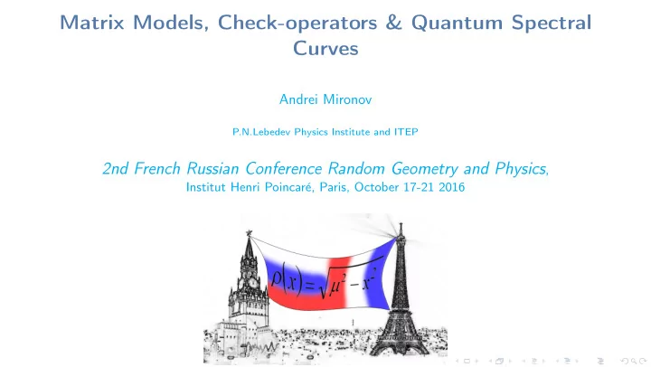
Matrix Models, Check-operators & Quantum Spectral Curves Andrei - PowerPoint PPT Presentation

Matrix Models, Check-operators & Quantum Spectral Curves Andrei Mironov P.N.Lebedev Physics Institute and ITEP 2nd French Russian Conference Random Geometry and Physics , Institut Henri Poincar´ e, Paris, October 17-21 2016

Plan Introduction Multiple solutions to the Virasoro constraints Check-operators Seiberg-Witten (SW) like solutions and integrable properties Quantum curves Quantum curves from degenerate conformal blocks Modular kernels in CFT A.Mironov (LPI/ITEP) Matrix Models,Check-operators, and Quantum Spectral Curves 2016 2 / 23

Old Story: Matrix Models: Virasoro constraints = loop equations = Ward identities + integrability New Story: Check Operators: The space of solutions to the loop equations + quantized Whitham flows An application: Strings: matrix model networks as a tool to study topological strings and Nekrasov functions. Algebraically: conformal blocks of Virasoro/W and Ding-Iohara-Miki algebras Quantum field theory: supersymmetric quiver gauge theories of Seiberg-Witten type A.Mironov (LPI/ITEP) Matrix Models,Check-operators, and Quantum Spectral Curves 2016 3 / 23

Two-parametric deformations of Seiberg-Witten (SW) systems: Integrable system Spectral curves Gauge theory conformal matrix models, KP hierarchy degenerate conf. block equation Nekrasov function ↓ ǫ 2 → 0 quantum SW system quantum many-body integrable system, � = ǫ 1 Schr¨ odinger (Baxter) equation ↓ ǫ 1 → 0 Seiberg-Witten system Spectral curve + Whitham flows classical finite-dimensional integrable system A.Mironov (LPI/ITEP) Matrix Models,Check-operators, and Quantum Spectral Curves 2016 4 / 23

Matrix integrals and check-operators Simplest example: the Hermitean matrix integral � Z = dM exp [ Tr V ( M ) ] where we parameterize � t k M k V ( M ) = k =0 Loop equations = Virasoro constraints: L n Z = 0 , n ≥ − 1 ∂ 2 ∂ � � L n = t k + ∂t k + n ∂t a ∂t b a + b = n ∂Z = NZ ∂t 0 A.Mironov (LPI/ITEP) Matrix Models,Check-operators, and Quantum Spectral Curves 2016 5 / 23

Solutions as formal series There is no solution such that Z is a power series! Gaussian case ( t 2 → t 2 − α ): � � − α Tr M 2 + Tr V ( M ) � = c 0 + c 1 t 1 + c (1) 1 + c (2) 2 t 2 Z = dM exp 2 t 2 + . . . The coefficients are constructed from � � − α Tr M 2 � M k dM exp c i ∼ α − i/ 2 which is evident by dimensional argument. A.Mironov (LPI/ITEP) Matrix Models,Check-operators, and Quantum Spectral Curves 2016 6 / 23

More general (Dijkgraaf-Vafa) case: � Z = dM exp [ Tr W ( M ) + Tr V ( M ) ] W ( M ) = � n T k M k , t k − → T k + t k in the Virasoro constraints. The coefficients are constructed from � dM exp [ Tr W ( M ) ] M k Z = i.e. there are combinations of T k ’s in denominators. How many solutions? Solutions are parameterized by an arbitrary function of n − 2 variables T k . Two of them are fixed by L 0 Z = 0 , L − 1 Z = 0 Thus, for n = 2 (Gaussian case) there is a unique solution. A.Mironov (LPI/ITEP) Matrix Models,Check-operators, and Quantum Spectral Curves 2016 7 / 23

More general (Dijkgraaf-Vafa) case: � Z = dM exp [ Tr W ( M ) + Tr V ( M ) ] W ( M ) = � n T k M k , t k − → T k + t k in the Virasoro constraints. The coefficients are constructed from � dM exp [ Tr W ( M ) ] M k Z = i.e. there are combinations of T k ’s in denominators. How many solutions? Solutions are parameterized by an arbitrary function of n − 2 variables T k . Two of them are fixed by L 0 Z = 0 , L − 1 Z = 0 Thus, for n = 2 (Gaussian case) there is a unique solution. A.Mironov (LPI/ITEP) Matrix Models,Check-operators, and Quantum Spectral Curves 2016 7 / 23

Technical tools: loop equations Generating functions of correlators = resolvents: � � 1 = 1 ρ (1) ( z ) = ∇ z Z = ˆ ˆ Tr ∇ z F z − M Z � � 1 1 ρ (2) ( z 1 , z 2 ) = = ˆ ∇ z 1 ˆ Tr z 1 − M Tr ∇ z 2 F z 2 − M c . . . where 1 ∂ � ˆ ∇ z = , Z = exp F z k +1 ∂t k k Loop equations: � L n [ T ( z ) Z ] − = 0 , T ( z ) ≡ z n +2 � � � � ρ (1) ( z ) 2 + ˆ ∇ z ρ (1) ( z ) + W ′ ( z ) ρ (1) ( z ) + W ′ ( z ) ρ (1) ( z ) V ′ ( z ) ρ (1) ( z ) + = 0 + − � �� � � �� � =0 as t k → 0 polynomial of degree n − 2 A.Mironov (LPI/ITEP) Matrix Models,Check-operators, and Quantum Spectral Curves 2016 8 / 23

Check-operator: acting on the space of solutions. � � ( a + b + 2) T a + b +2 z a ∂ � + ≡ ˇ ˇ W ′ ( z ) ρ (1) ( z ) f n − 2 ( z ) = R z F , R z = − ∂T b a,b Classical spectral curve: Genus expansion: � 1 t k , T k → 1 g t k , 1 � � g 2 k F k g T k , Z = exp g 2 F , F = k Leading term of the genus expansion: ρ (1) ( z ) = − W ′ ( z ) + y ( z ) 2 where y ( z ) 2 ≡ W ′ ( z ) 2 − 4 f n − 2 ( z ) determines the classical spectral curve. A.Mironov (LPI/ITEP) Matrix Models,Check-operators, and Quantum Spectral Curves 2016 9 / 23

Examples: Gaussian case: n = 2 , f 0 ( z ) = const , y 2 = z 2 − const : semi-circle distribution. W 3 -case: n = 3 , f 1 ( z ) is a linear function, the spectral curve is a torus, the space of solutions is described by a function of one variable. Meaning: typical integration in the matrix (eigenvalue) integral � dxe W 3 ( x ) implies two independent choices of contour (Airy functions). N eigenvalues in the integrand part into two groups (two contours), N 1 and N 2 , N 1 + N 2 = N . This describes the two-cut solution (torus). Arbitrary function of one variable corresponds to one arbitrary variable, fraction N 1 /N 2 . A.Mironov (LPI/ITEP) Matrix Models,Check-operators, and Quantum Spectral Curves 2016 10 / 23

Summary of general properties: 1. Any solution is unambiguously labeled by an arbitrary function of n − 2 T -variables: the bare F (0) ( T ) . 2. Solutions of the Virasoro constraints (or loop equations) are constructed from F (0) ( T ) by an evolution operator ˆ U ( T, t ) that does not depend on F (0) ( T ) : U ( T, t ) e F (0) ( T ) Z ( T, t ) = ˆ 3. The evolution operator can be completely expressed in terms of the unique operator � ( a + b + 2) T a + b +2 x a ∂ � W ′ ( x ) 2 − 4 ˇ ˇ y ≡ ˇ R ( x ) , R ( x ) ≡ − ∂T b a,b =0 its derivatives and W ′ ( x ) . A.Mironov (LPI/ITEP) Matrix Models,Check-operators, and Quantum Spectral Curves 2016 11 / 23

Consequence: ρ (1) ( z ) = ˆ ∇ z ( t ) F = ˇ ∇ z ( T ) F The main check-operator ˇ ∇ z is expressed through y , its derivatives and W ′ ( x ) . Important: [ ˆ ∇ z 1 , ˆ ∇ z 2 ] = 0 , but [ ˇ ∇ z 1 , ˇ ∇ z 2 ] � = 0 . Main property: � � dz ˇ dz ˇ [ ∇ z , ∇ z ] = δ ij A i B j y 2 = W ′ 2 ( x ) − 4 ˇ R ( x ) F (0) . The curve: A.Mironov (LPI/ITEP) Matrix Models,Check-operators, and Quantum Spectral Curves 2016 12 / 23

DV/SW system: � � � A i dz ˇ A i dz ˇ A i dzρ (1) ( z ) = a i , then Choose the basis of eigenfunctions ∇ z Z a = a i Z a , i.e. ∇ z F a = � dzρ (1) ( z ) = ∂ F ∂a i B i N i are associated with � ρ (1) ( z ) dz a i = A i Integrable properties: Z N ( t ) is a τ -function of the Toda chain (as a formal series) Z DV ( T, N i ) is the SW system; it satisfies the Whitham hierarchy in the planar limit, T i are Whitham flows. A.Mironov (LPI/ITEP) Matrix Models,Check-operators, and Quantum Spectral Curves 2016 13 / 23

Quantum spectral curve: The Backer-Akhiezer function: Ψ BA ( z ) = e V ( z ) / 2 Ψ( z ) where � � 1 Ψ( z ) = Z t k − 1 � z dξ ˆ ∇ ξ = � det( z M ) � kz k Z ( t ) z N e = Z ( t ) and < ... > means the matrix model average. From the Virasoro constraints the quantum spectral curve: � � z + V ′ ( z ) ∂ z + ˇ ∂ 2 R z Ψ( z ) = 0 In the limit, ∂ log Ψ( z ) = ρ (1) ( z ) it turns into the classical spectral curve (planar loop equation): ρ (1) ( z ) 2 + V ′ ( z ) ρ (1) ( z ) + ˇ R z F = 0 The equation for the Baker-Akhiezer function looks as � � z − 1 2 V ′′ ( z ) + 1 4 V ′ ( z ) 2 − 1 2[ ˇ R z V ( z )] + ˇ ∂ 2 R z Ψ BA ( z ) = 0 ˇ R z contains the derivatives w.r.t. the Whitham times. A.Mironov (LPI/ITEP) Matrix Models,Check-operators, and Quantum Spectral Curves 2016 14 / 23

AGT and conformal blocks: quantum spectral curve Conformal block: G ( x, ∆; ∆ i , c ) , ∆ = ( Q − α ) α , c = 1 + 6 Q 2 , Q = b − 1 /b , V α ( z ) = e iαφ ( z ) . Degenerate field: ( b 2 L 2 − 1 − L − 2 ) V 1 / 2 b ( z ) is a primary field, i.e. V 1 / 2 b ( z ) is degenerate at the second level. The equation for the 5-point block with the degenerate field at z :     z + (2 z − 1) ∂ z − q ( q − 1)   b 2 z ( z − 1) ∂ 2 z − q ∂ q + rational function of q G 5 ( z | 0 , q, 1 , ∞ ) = 0       � �� � check-operator This is the quantum spectral curve, q is a counterpart of T k . A.Mironov (LPI/ITEP) Matrix Models,Check-operators, and Quantum Spectral Curves 2016 15 / 23

Comment. In the limit when all ∆ i → ∞ , this equation is reduced to the non-stationary Schr¨ odinger SU (2) periodic Toda chain equation: � � z − 2Λ 2 cosh z + 1 ∂ ∂ 2 G T oda = 0 5 4 ∂ Λ where Λ is the limit of rescaled q . log Λ is known to play the role of the first Whitham time in the Seiberg-Witten theory. A.Mironov (LPI/ITEP) Matrix Models,Check-operators, and Quantum Spectral Curves 2016 16 / 23